
This tutorial will help you to learn the basic information needed to run an optimisation study in DesignBuilder in a few easy steps.
Create a new file located in London Gatwick and add a building to the site with a simple rectangular block having dimensions 30m x 20m as shown below. Use default Model options and template settings. DesignBuilder as supplied will use a Simple HVAC Fan Coil Unit system as the default. For this example you should make sure that you have heating and cooling selected and no natural ventilation (this will be the case for a new model with a FCU HVAC system selected).
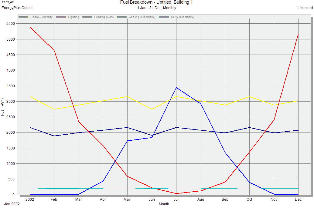
Click on the Simulation tab and run a base annual simulation. Because it is a simple model you can select hourly results. Make sure to also choose Monthly results which are required by the Optimisation. Check the hourly results for the simulation period and make sure that the model is behaving as expected, including temperatures within the building, operations periods etc. If not fix the model and repeat this step until you are happy with the base model hourly results. Monthly results should something like the screenshot below.
Once you have a good understanding of how the base model operates, you are ready to start the optimisation stage. To do this click on the Optimisation tab on the Simulation screen. Because you don't have any results yet the Optimisation Analysis Settings dialog is displayed. This allows you to define the optimisation problem, i.e. what it is that you want to achieve from the optimisation study. Use the default settings for this simple example which request an optimum set of solutions to minimise both operational construction emissions and discomfort allowing for variations in window to wall ratio and heating and cooling setpoint temperatures.
Objectives:
Constraints:
None
Design variables:
Allow WWR and cooling and heating setpoints to vary as shown in the screenshot below. Variations are made at building level for all variables in this case as shown by the Target objects column.

The only change that may be required is to change the minimum Cooling setpoint temperature to have a value of 23.1. All other settings described so far are defaults for a new model.
Having confirmed the Optimisation analysis options the next dialog to open will be the Optimisation calculation options. Change the Initial population size to 10 for this small analysis and otherwise use default settings.
Once you have completed your review of the options press the Start button in the bottom right of the screen. The optimisation process will involve running a lot of simulations. With the recommended settings there will be 100 generations with a population size of at least 10 in each, growing as Pareto solutions are added. That means that at least 100 x 10 = 1000 simulations will be run! For our simple model and when using the Simulation manager to run these in parallel this shouldn't take too long. However if time is an issue it is usually worth keeping an eye on the solutions as they come in to check whether convergence has been achieved.
While preparing this tutorial we made the judgement that the solution was effectively converged after 76 generations and pressed the Stop button at that point. If the optimisation had been left to continue the red Pareto front line would probably have been filled in further however this would not provide much extra information for the purposes of our example test. After pressing Stop the current generation continues to simulate and once that is finished we see a graph like that below.

Try using some of DesignBuilder's analysis tools to investigate the best settings in this case.
Next steps to learning. Try adding more design variables. Glazing type, shading systems etc. Try using some other variable types.