To start an optimisation analysis go to the Simulation screen and click on the Optimisation tab. Calculations are updated using the Update toolbar icon in the usual way. The data on the Optimisation Calculation Dialog is used to provide options to control the optimisation analysis as well as outputs to help you to understand the progress being made as the calculations continue.
Note: It is important to run the base simulation with monthly/annual outputs before opening the optimisation tab. The optimisation simulations will all be run using the base calculation and model options.
The genetic algorithms (GA) used by DesignBuilder require a number of options to control the way that the solutions evolve.
Enter a description for the calculation. This text will be used to identify the results on the graph and any other related outputs.
Under the headers for the 4 objective functions you can enter the minimum and maximum values to be considered when evaluating the success of a design variant. You should not change the checkbox settings under Objective functions.
During the optimisation process each design variant to be tested is scored for overall success based on the value of the Objective KPI for the design. The score for each objective is calculated as:
Objective score = KPI Value / KPI ValueMax
The overall success score for the design variant is derived by combining the scores for each individual objective as follows:
Success score = √ Σ Objectives KPI Values 2
The Success score can be thought of as the Euclidean distance from the origin to the of the point on the corresponding Pareto plot.
Note: Because the maximum objective function values are used as part of the scoring mechanism they are important inputs.
The objective function maximum values can be used to control the weight given to each objective in the scoring equation above. This will have an influence the evolution of the population. Assigning a higher maximum value to an objective function (to be minimised) will tend to reduce the significance of that objective in the overall score. (high KPI ValueMax means low Objective score)
Likewise reducing the maximum value increases the significance of the objective relative to that of other objectives.
Because it is so important to select appropriate maximum objective values it is usually worth running a few generations in a test analysis to assess the range for each objective function. Then use the resultant partial graph to decide on a maximum value for each objective. Because the partial analysis probably didn't explore much of the design space it is usual to add a safety margin to the actual recorded maximum values generated. For example if the maximum carbon emissions in the preliminary analysis came out as 30,000,000 kg then you might set the carbon emissions objective maximum value to 40,000,000 kg.
Once you have decided on good values to use, stop the analysis, enter the new maximum objective function values, reset results and restart the analysis with appropriate maximum values.
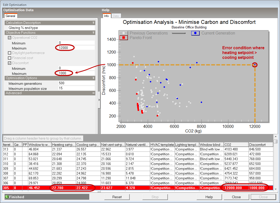
Some designs are considered invalid. For example in a controls analysis it is not normally allowed for heating setpoint temperature to be higher than cooling setpoint temperature. If a particular design variant has an invalid configuration then it is assigned a bad score using the maximum objective score (assuming objectives are being minimised). This discourages similar invalid design variants from appearing in future generations.
The screenshot below illustrates how DesignBuilder handles invalid design variants by applying the maximum objective function values.
Note: If you enter a maximum value that is smaller than all design values then this can at least reduce the efficiency of the optimisation process and at worst cause optimisation results to be inaccurate. This is because any erroneous designs will be given scores of the maximum objective value, but if the maximum objective value is actually smaller than the values calculated then the invalid designs could become Pareto optimal! This will tend to encourage more similar designs, increasing the number of bad designs in the gene pool.
The maximum number of generations to be used will determine the time/computing resources required to complete the analysis. The value entered here will usually reflect the complexity of the analysis. The default value for maximum generations is 200 and typical values are in the range 50-500. You can of course set a larger number at the beginning, and then manually terminate the search process when sufficient good solutions have been found.
Each generation will include at most this number of designs. The bigger the population size, the more different solutions may exist within the same generation. Larger population sizes may be required for problems containing 5 or more design variables. The default maximum population size is 15.
The number of bits used to define each float (numeric) design variable value. The number of options this gives rise to can be calculated as 2n, where n is the encoding length. This value should normally be between 6 and 14. An encoding length of 10 for a float gives 1024 equally spaced samples within the specified range of the design variable. This in most cases will be adequate.
The number of bits used to define each list design variable value. The maximum number of options that this option can accommodate can be calculated as 2n,where n is the encoding length. For example a value of 6 allows up to 26 = 64 items per list. If you have less than 64 items in each variable list then a value of 6 should be a good choice here.
The “Tournament operator” is used in this implementation of Genetic Algorithm for selecting better solutions from the current generation. Tournament size means the size of a random sample taken in the current generation. From this random sample, the best solution will be selected for “reproduction”. Default value is 2.
This rate is in fact a relative probability (compared to individual mutation probability) of a new solution being created by crossover. For example, if the crossover rate is 1.0 and individual mutation probability is 0.5, there are 67% (1.0/1.5) of chance the new solution will be created by crossover, and 33% (0.5/1.5) of chance it will be created by mutation.The default value is 0.9. Typical range is 0.6-1.0
Check this option if you wish to override the default value of bitwise mutation probability. The defaults value is 1/nbits where nbits is the total of the number of bits in the chromosome calculated by summing the number of bits for each variable. For numeric variables the number of bits is the Encoding length for floats and for list variables the number of bits is the Encoding length for lists. The maximum default value is 0.1 and the minimum is 0.01.
If you choose to override the automatic calculation then the value can be entered here.
See crossover rate. Default is 1.0.
When 2 objective functions are defined, the trade off for the range of design variables considered is displayed graphically on the scatter graph. The Pareto optimal solutions are displayed in red, current generation are shown in blue and previous generations are shown in dark grey.
When a single objective is used the graphical output shows the evolution of the objective function for each iteration. Because there is no trade off with single objective optimisation, only the single most optimal solution is highlighted in green in the grid.