The genetic algorithms (GA) used by DesignBuilder require a number of options to control the way that the solutions evolve.
Enter a description for the calculation. This text will be used to identify the results on the graph and any other related outputs.
The maximum number of generations to be used will determine the time and computing resources required to complete the analysis. The value entered here will usually reflect the size and complexity of the analysis. Typical values are in the range 50-500 depending on size of the problem, the population size and whether a Pareto archive is used.
You can set a larger number of generations at the beginning, and then manually terminate the search process when sufficient good solutions have been found.
Tip: When seeking accurate optimal outputs and hence using a large value for Maximum generations it can be worth experimenting with higher mutation rates to help avoid early convergence.
Each generation will include at least this number of designs. The bigger the population size the more different solutions may exist within the same generation. Larger population sizes may be required for problems containing 5 or more design variables or where some variables have many options.
Note: All simulations for a generation must complete before the next generation is started so if you have many parallel cores at your disposal and the time taken to run the simulations is the main bottleneck then a higher number here can be helpful.
This option allows you to only display feasible solutions on the Pareto Front. Solutions failing one or constraint requirement are not included on the Pareto Front. This option applies to the graphic display of the Pareto Front only and does not affect the solution itself. The option can be changed during the simulation.
Checking this option shows on feasible solutions and hides all other solutions failing one or more constraint requirement.
Check this option if the optimisation is to include a Pareto archive to feed previously identified "best so far" solutions into the population to encourage exploration around previously identified Pareto optimal designs. This option can help the solution to progress more quickly. On the other hand it can also lead to early convergence so some experimentation may be required to find the best setting for each new analysis.
When using a Pareto archive you must also define an upper limit on the population size including both the standard population and the Pareto Front archive. The default maximum population size is 50.
The number of bits used to define each float (numeric) design variable value. The number of options this gives rise to can be calculated as 2n, where n is the encoding length. This value should normally be between 5 and 10. An encoding length of 10 for a float gives 1024 equally spaced samples within the specified range of the design variable. In most cases a value of 6 (the default) will be adequate giving 64 samples.
The interval size is calculated as (objective max value - objective min value) / (2n - 1).
The “Tournament operator” is used in this implementation of Genetic Algorithm for selecting better solutions from the current generation. Tournament size means the size of a random sample taken in the current generation. From this random sample, the best solution will be selected for “reproduction”. Default value is 2.
This rate is in fact a relative probability (compared to individual mutation probability) of a new solution being created by crossover. For example, if the crossover rate is 1.0 and individual mutation probability is 0.5, there are 67% (1.0/1.5) chance that the new solution will be created by crossover, and 33% (0.5/1.5) chance it will be created by mutation. The default value is 1.0. Typical range is 0.6-1.0
It is important to avoid "premature convergence" where the optimisation settles on a Pareto front which is incomplete or inaccurate. The Individual mutation probability helps to maintain diversity in the population to ensure that the parameter space is fully explored which in turn helps to avoid premature convergence and missing the full set of optimal solutions.
Low values of Individual mutation probability (e.g. 0.2) can help to avoid wasting time exploring non-optimal parts of the parameter space which leads to fast convergence; however the results may not be as accurate as when using higher values. DesignBuilder uses a balanced default of 0.5.
See also Crossover rate.
Check this option if you wish to override the default value of bitwise mutation probability. The default value is 1/nbits where nbits is the total of the number of bits in the chromosome calculated by summing the number of bits for each variable. For numeric variables the number of bits is the Encoding length for floats and for list variables the number of bits is the Encoding length for lists. The maximum default value is 0.5 and the minimum is 0.01.
If you choose to override the automatic calculation then the value can be entered here.
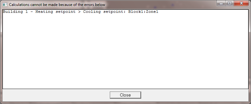
It is important to understand the cause of any errors that occur during an optimisation. The Pause on errors option, when checked, causes a message to be displayed and the optimisation is paused. For example if there is an overlap in heating and cooling setpoint temperatures, in configurations where the heating setpoint is higher than the cooling setpoint the following error message is displayed:
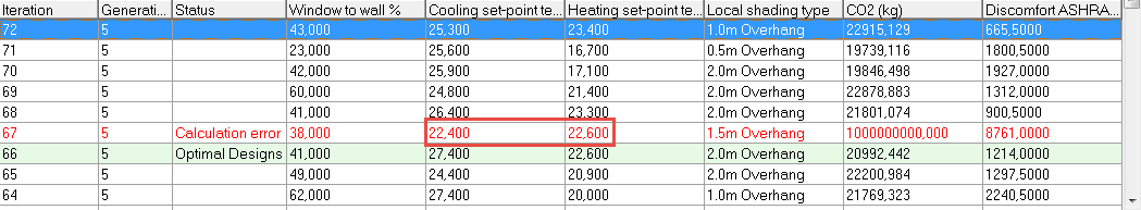
This sort of error does not cause a problem for the overall optimisation study. If a particular design variant has an invalid configuration then it is assigned a penalty using the maximum objective score (assuming objectives are being minimised). This applies evolutionary pressure to discourage similar invalid design variants from appearing in future generations.
Once you are clear about the cause of nay errors you will normally want to stop seeing reports and allow the optimisation to continue. To do this simply uncheck this check box. Designs with errors are displayed in red in the grid as shown below.
Common causes of errors are:
An important and often overlooked consideration is the impact of the time taken by DesignBuilder to generate the IDF input file for each design. The longer this is relative to simulation time the greater the model generation bottleneck and the less useful the large number of parallel simulations. On the other hand, the larger and more complex the model and the more detailed the simulations (nat vent, detailed HVAC, more time steps etc) the more time is taken in simulation and relatively less in IDF generation. For an extremely large/complex model, all IDF inputs will have been generated before the first results are in and the large number of parallel simulations will speed progress. For a smaller model, the IDF generation bottleneck is more significant and first simulation results will be in before the 3rd or 4th IDF input has been generated and in this case the multiple cores will not be needed. This is often the case for simple single zone models. To test and understand this watch the Simulation Manager while the optimisation takes place. You will see new jobs being submitted, queued and simulated.
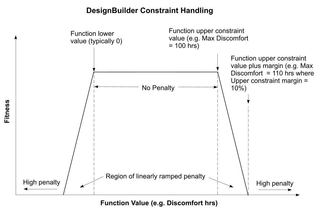
The lower and upper constraint margins are used as part of the constraint handling method used by DesignBuilder, which is based on a generic penalty function approach. During a constrained optimisation each design alternative is tested against any constraints applied and a penalty is generated based on whether the design is feasible or not, i.e. whether it meets constraint requirements. If the function value is within the feasible range then no penalty is applied and conversely if it is outside the feasible range then a penalty is applied. There is a margin between the feasible and the infeasible regions where a linearly ramped penalty is applied. The upper and lower margins set on the Calculation options dialog are used to define these regions as shown on the graph below.
When 2 objective functions are defined, the trade off for the range of design variables considered is displayed graphically on the scatter graph. The Pareto optimal solutions are displayed in red, current generation are shown in blue and previous generations are shown in dark grey.
When a single objective is used the graphical output shows the evolution of the objective function for each iteration. Because there is no trade off with single objective optimisation, only the single most optimal solution is highlighted in green in the grid.