
This internal CFD example will guide you through the basic minimum steps required for an internal CFD analysis:
The model comprises a simple rectangular block housing a zone with dimensions 6.0m x 4.0m x 3.5m.
Create a new site and add a new building using default settings. From the building level Click on the ‘Add new block’ tool and change the “Block type” to “Building block”, the “Height” to 3.5m and set the wall thickness to 0.25m.
Default wall and window boundary temperatures can be defined from the building level down to the surface level. As with other DesignBuilder attribute data, these attributes are inherited from the level above unless deliberately overwritten.
The default wall and window boundary temperatures can be accessed under the CFD Boundary header on the CFD tab of the model data.
At the building level, change the default window temperature to 20°C.
Go down to the zone surface facing North and change the default wall temperature to 18°C and the default window temperature to 10°C. Go through the same procedure for the west facing zone surface.
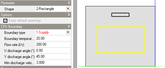
A 0.5m x 0.5m extract grille is to be located in the corner of the ceiling 0.5 m from the North and east surface edges.

Click on the building in the navigator to move to the building level and click on the CFD tab to set up an internal CFD analysis. An internal analysis can be set up for any level from a single zone up to the whole building. In this case, because we are dealing with a single zone building, the analyses for each level would be identical. After clicking on the CFD tab, the New CFD analysis dialog is displayed. Enter Basic Vent in the Name field and leave the grid spacing and grid line merge tolerance at their default settings. More on grids in the next exercise.
Click OK to create the analysis data set.
You will see the model in wire-frame mode by default and at this stage the CFD analysis has been created including the default grid and the model is ready for calculations. If you were going to edit the grid now is the time – before starting the calculations, but for now we will use the default grid.
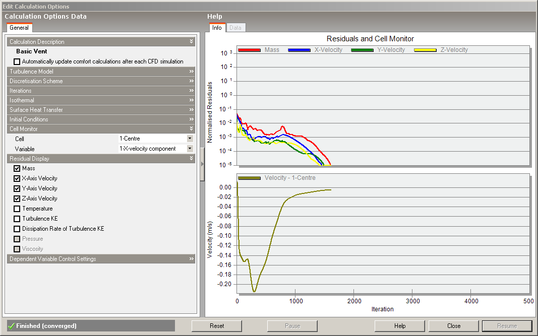
To set up calculation data and run the CFD calculations, click on the “Update calculated data” button, which will bring up the CFD Calculation options dialog. The left hand side of the calculation dialog contains various calculation options. Keep the default options except under the Residual Display header, switch on the X, Y and Z-axis velocity residuals.
Click on the Start button to begin the calculations. Wait until the calculation is fully converged when the residuals have reached the specified minimum (1x10⁻⁵ is the default for all variables) and the Finished (Converged) indicator is displayed at the bottom left of the dialog. Notice that the displayed velocity for the default Centre monitor point becomes constant (bottom graph).
Press the Cancel button to close the calculation dialog.
After the calculations have been completed, the CFD results display options data panel is enabled allowing you to set various results display options. Use default Display options.
Click on the Select CFD slice tool. Click on the Y-axis of the grid axis selector (top right of screen) and then move the cursor over the ceiling surface along the Y-axis to move the slice selection frame midway between the North and South-facing walls, 2.0m from each wall and click the mouse button to add the currently selected slice to the display.

Notice that as you move the slice selection frame to a slice that was previously added to the display, the frame colour changes from green to red and if you click the mouse button, the slice is removed from the display.
Try adding more slices in other planes to see the key characteristics of temperature and velocity distribution in the zone.
Press the ESC key to cancel Select CFD slice tool.