
In this second internal CFD exercise, the model is modified to include radiators as well as the supply and extract vents entered in the first tutorial. Also some more advanced features of the CFD calculations and display are explored. You will learn how to:
Assemblies consist of 1 or more component blocks combined and are used to create boundary conditions inside or outside blocks. They can be used to create furniture, heat generating equipment, airflow supply and extract etc.
In this exercise a radiator assembly is to be created from a single component block, which is to be drawn using a rectangular extrusion.
To convert the component block to an assembly and add the resulting assembly to the model assembly library:

Assemblies inside the building must be placed at Block level (not zone level) so to place a radiator assembly first click on the block in the navigator to move down to the block level.
To position assemblies accurately you must use construction lines.
To do this, orbit the model to get a clear view of the west-facing end wall from the inside of the block and then click on the Place construction line tool.
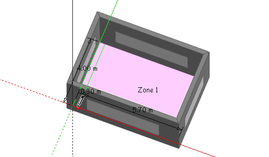
To position the construction line accurately, switch on the Increment snap under Point Snaps on the Drawing Options data panel. Move the cursor to snap to the lower surface edge at the bottom of the North-facing wall and move the cursor to obtain an edge snap 0.3m from the end nearest the west-facing wall. Click the mouse to start the construction line and move the mouse to the opposite edge at the bottom of the South-facing wall, snapped to the Y-axis and click the mouse once the edge snap is established on the opposite edge to place the construction line.
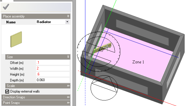
Click on the Place assembly tool and as you move the cursor back across the Edit screen, you will see that a copy of the previously created radiator assembly is attached to the cursor and the Place assembly data panel is displayed at the bottom left of the screen. Set the Offset to 0.1m to offset the base of the radiator 0.1m above the floor level, set the Width to 2.0m, the height to 0.6m and leave the Depth at 0.06m. Move the cursor to establish a snap on the construction line and click the mouse to place the radiator origin. Once the radiator has been placed, a protractor is displayed at the assembly origin enabling you to define the rotation. Rotate the radiator assembly until it is parallel with the nearest wall and then click the mouse to set the rotation.
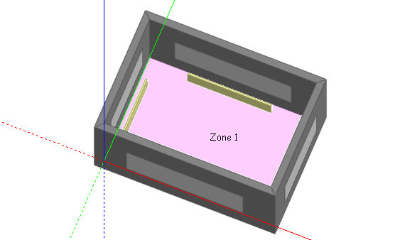
Repeat this procedure to place a 3.0m radiator adjacent to the North-facing wall.
We are now ready to start a new CFD calculation so again click on the building in the navigator to move to the building level and click on the CFD tab. If you have just finished the first CFD exercise, the analysis results for these calculations will be displayed. You should now create a new analysis because the model has changed with the addition of the radiators. To do this click on the CFD Results Manager toolbar icon. This displays the dialog below.

Note that the first Basic Vent analysis is flagged as not up-to-date. This is because the model has been edited since the last calculation was made.
Click on the New button to create a new analysis using the model in its current state. The New CFD analysis dialog is displayed. Enter Radiators and Vent in the Name field and leave the default grid spacing and grid line merge tolerance at their default settings. The default grid spacing and grid line merge tolerance are used in generating the CFD grid. During the process of creating a new CFD analysis data set, a 3-D CFD grid is automatically generated by extracting key points from the model geometry along each of the major axes. The spaces between the key points are known as grid regions and are automatically divided into sub-regions using the default grid spacing entered on the Calculation options dialog. The grid line merge tolerance enables key point grid lines that are very close together to be merged in order to prevent very high aspect ratio cells from being created which can lead to calculation instability.
Click OK to create the analysis data set.
You will see the model in wire-frame mode by default and at this stage the CFD analysis has been created including the default grid and the model is ready for calculations.
But before starting the calculations we will explore the edit grid capability. First click on the Edit CFD grid tool. Move the cursor across the displayed CFD grid to select grid regions along the current grid axis. Selected grid regions are highlighted in cyan.
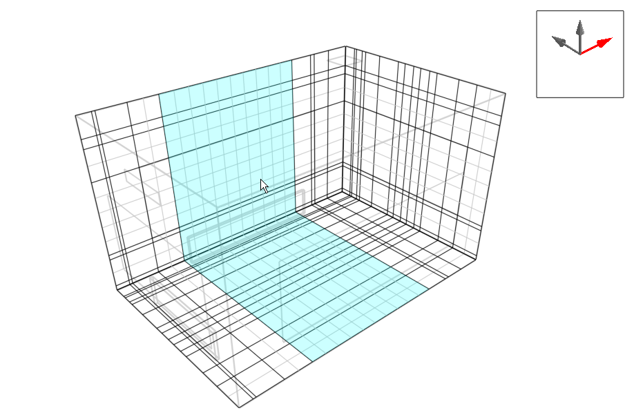
To change the current grid axis, click on one of the major axes in the grid axis selector tool that is displayed at the top right of the CFD screen. To edit a selected region, click the mouse on the currently selected region. The selected region will turn red and the Edit CFD grid region data panel will be displayed at the bottom left of the screen. You can select Edit region from the Operation drop list to change the default spacing of the region or Insert region to create a new region and in the case of a previously inserted region, you can select Remove region to remove it.

To cancel the Edit CFD grid tool press the <Esc> key.
After editing the default grid, you can reset it to the default by clicking on the Reset CFD grid tool. Also, to obtain information about the grid, you can click on the Show CFD grid statistics tool which brings up a dialog indicating the number of cells, required memory, available memory and maximum cell aspect ratio.
For the purpose of this tutorial, the default grid will be used.
In order to monitor the convergence of the solution, it can be useful to set up a number of monitor points throughout the calculation domain. During the calculation it is then possible to enable a plot of the variation of the various dependent variables for each of the defined monitor points in order to see if the variables have reached a constant value as the CFD calculation proceed.

When a monitor cell has been added, a cell marker is displayed together with the cell name.

You can press <Esc> to cancel the Define CFD monitor points tool.
To set up calculation data and run the CFD calculations, click on the Update calculated data button, which will bring up the CFD Calculation options dialog. The left hand side of the calculation dialog contains various calculation options. Keep the default options except under the Residual Display header, switch on the X, Y and Z-axis velocity residuals.
Click on the Start button to begin the calculations. Wait until the calculation is fully converged when the residuals have reached the specified minimum and the “Finished (Converged)” indicator is displayed at the bottom left of the dialog. Notice that the displayed velocity for the default Centre monitor point becomes constant (bottom graph).
In the CFD results slices, velocity vectors are displayed as arrows, the length of which corresponds to the magnitude of the velocity and with the default vector scale factor of 1.0, a length of 1.0m corresponds to a magnitude of 1.0m/s. The maximum vector length is the maximum length of a vector that will be displayed to prevent the display from becoming cluttered with excessively large vectors. Any vector, which has a magnitude greater than this maximum, will be displayed translucently to distinguish it from vectors with lengths that do represent magnitude.
The default minimum and maximum dependent variable values are extracted from the minimum and maximum values found in the domain and this range is then divided into twelve equal increments in order to arrive at the dependent variable contour bands. Each contour band can be edited or switched off altogether.
In this tutorial the maximum temperature will be 75.0°C (the temperature of the radiators), which is well above the mean temperature of the space, and consequently the default contour bands would be far from the mean and the resulting display would not be very informative. So in order to compress the contour bands to be within the likely temperature range throughout the domain DesignBuilder automatically sets the Maximum Temperature under temperature bands range to 24.0°C and the minimum value to 18°C.
You can manually change these maximum and minimum values in the Display options panel. Note that you need to click on the green tick Apply changes button in order for the display attributes to take effect. Notice also that the temperature contour bands are updated using the new temperature range.
You can revert to the absolute minimum and maximum values in the model by using the Tools > Reset CFD display variables menu command.
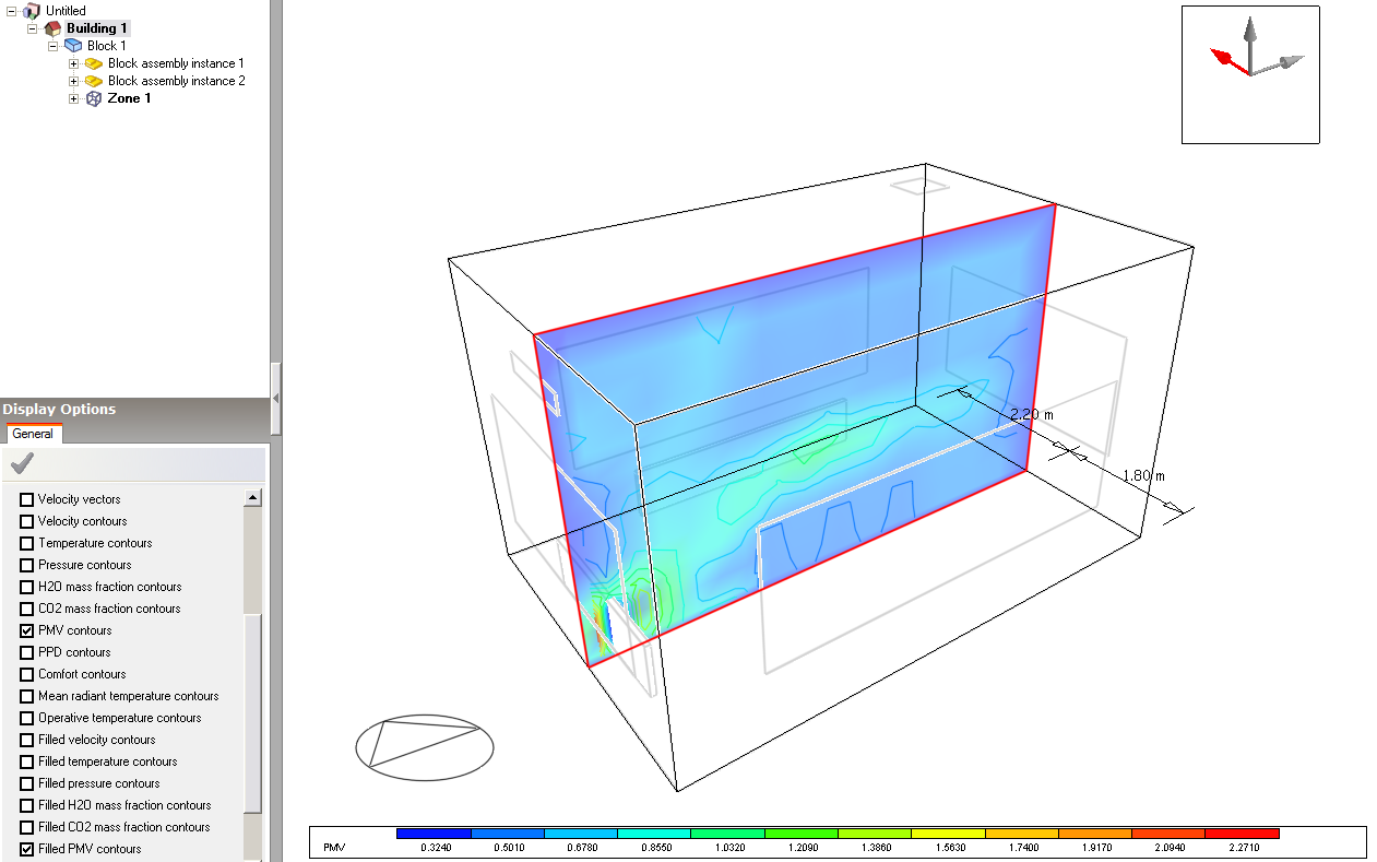
Click on the Update CFD comfort tool to carry out comfort calculations. After the calculations have been completed, various comfort variables are available for display, PMV, PPD, operative temperature and mean radiant temperature. Clear all slices from the display using the Clear all slices tool. Switch off Velocity vectors and Filled temperature contours under the Slice Settings header on the Display options panel and switch on the PMV contours and Filled PMV contours. Click on the green tick Apply changes button.
Click on the Select CFD slice tool and click on the Y-axis of the grid axis selector. Move the cursor over the ceiling surface along the Y-axis to move the slice selection frame again to be midway between the North and South-facing walls and click the mouse button to add the slice to the display.
You can now switch between the 2 CFD analyses you have carried out using the CFD Analysis Manager dialog. Select the analysis you wish to switch to and use the Open button to load results. Any slices associated with the analysis will be restored. These 2 analyses will be stored in the dsb file by default and are not deleted when changes are made to the model.