The calculation method requires that the geometric space across which the calculations are to be conducted is first divided into a number of non-overlapping adjoining cells which are collectively known as the finite volume grid.
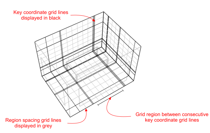
When a CFD project is created, a grid is automatically generated for the required model domain by identifying all contained model object vertices and then generating key coordinates from these vertices along the major grid axes. These key coordinates, extended from the X, Y and Z-axes across the width, depth and height of the domain respectively are known as ‘grid lines’. The distance between grid lines along each axis is known as a grid ‘region’ and these regions are initially spaced employing user-defined default grid spacing in order to complete the grid generation. The grid used by DesignBuilder CFD is a non-uniform rectilinear Cartesian grid, which means that the grid lines are parallel with the major axes and the spacing between the grid lines enables non-uniformity.
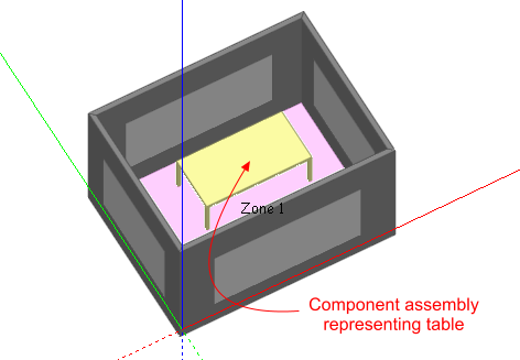
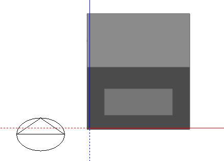
For example, looking at a simple building block with a single component assembly representing a table:
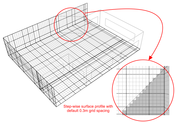
The resulting grid, generated with 0.3m default grid spacing would be as follows:
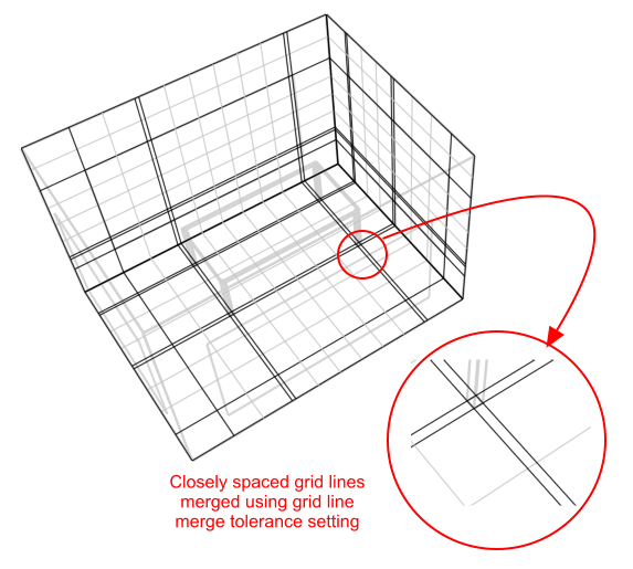
By default, grid regions are spaced uniformly using a spacing that is calculated to be as close to the user-defined default grid spacing as possible. Notice the narrow regions created between key coordinates associated with the tabletop and table legs. In this case, the distance between these key coordinates is of an acceptable value. However, very narrow regions resulting in long narrow grid cells or cells having a high aspect ratio should be avoided, as they tend to result in unstable solutions that can fail to converge. Highly detailed component assemblies can result in very large numbers of closely spaced key coordinates resulting in cells having high aspect ratios. Large numbers of key coordinates can also lead to overly complex grids and correspondingly high calculation run times and excessive memory usage which can be avoided by replacing very detailed assemblies with cruder representations for the purpose of the CFD calculation. However, where very narrow grid regions are unavoidable, adjacent grid lines formed from key coordinates can be merged together using the merge tolerance setting which is accessed through the new CFD analysis dialogs (see the Setting Up a New External CFD Analysis and ‘Setting Up a New Internal CFD Analysis’ sections). For instance, in the above example, if the table assembly had been located closer to the edge of the adjacent window, this could result in unacceptably close grid lines:

These closely spaced grid lines can be merged by creating a new analysis and increasing the grid line merge tolerance setting to say 0.025m:
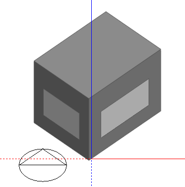
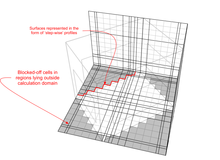
Due to the strict rectilinear nature of the grid, grid cells that lie in regions outside of the domain required for calculation are ‘blocked-off’ in order to cater for irregular geometries. It is important to take this into account when creating a model in order to maximise the efficiency of grid generation and/or to ensure that surface CFD boundaries will lie in the plane of a major grid axis to achieve accuracy of boundary representation. In some cases, the model may be rotated in order to ensure that most of the wall surfaces are orthogonal with respect to the grid axes. To take an extreme example, if a simple rectangular space has been drawn at a 45° angle to the Z-axis:
The resulting grid, generated using 0.3m default grid spacing, contains a great deal of redundancy in the form of blocked-off regions and inaccuracy of surface representation:
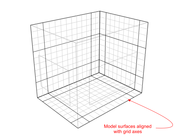
If the block is first rotated, to be aligned with the X-axis:
The resulting grid exhibits no redundancy and there is no inaccuracy in surface representation:
The accuracy of the representation of non-orthogonal surfaces can be improved by using smaller default grid spacing and in some cases specific grid regions can be modified to increase accuracy in a more localised fashion as illustrated by the following example:

Grid generated using default 0.3m grid spacing:
Using the ‘Edit CFD Grid’ tool, the grid spacing within just the regions spanning the angled section is reduced to 0.2m to improve the representation:

Grid regions between key coordinates can also be spaced using non-uniform spacing options and additional key coordinate regions can be added. Further information is provided on grid modification in the ‘Editing the CFD Grid’ section.