Accessed from Optimisation Calculation Options Dialog
The genetic algorithms (GA) used by DesignBuilder require a number of settings to control the way that the solutions evolve. These and other settings are made on the General tab of the Calculation Options dialog as described below.
The engine used in for optimisation is JEA - a powerful optimisation engine developed by EnSims.
Enter a description for the calculation. This text will be used to identify the results on the graph and any other related outputs.
The Start date set up for the base simulation on the analysis screen is displayed but cannot be edited here.
The End date set up for the base simulation on the analysis screen is displayed but cannot be edited here.
The number of solutions to be evaluated in each generation. The first-generation simulations are selected at random but form the basis of subsequent optimisation generations. More design variables require a larger population size in general. The choice may also be influenced by the number of processor cores you have for running these simulations. The default value is 15.
Tip: The Generation population size will typically be between 10 and 50 depending on the size of the analysis. For 3 design variables with say 10 options each then choose an initial population size of between 10 and 20. For 10 variables, each with 10 options then choose a value between 20 and 50. Like other settings on this dialog, the best values to use for the fastest and most reliable convergence will come from experience. In the meantime, a value of 15 will work well for most typical applications.
Note: All simulations for a generation must complete before the next generation is started so if you have many parallel cores at your disposal and the time taken to run the simulations is the main bottleneck in calculations (as opposed to IDF generation) then a higher number here can be helpful.
This option is used to decide when to stop the optimisation simulations. As the optimisation process progresses and most optimum solutions have been identified, fewer and fewer new optimal solutions will be found and there comes a point when it's time to stop. At the end of each generation, DesignBuilder checks whether any new optimal solutions were found in the most recent Generations for convergence generations. If so, the simulations continue, otherwise the optimisation process is considered to be complete, and results are displayed. It isn't possible to be sure that no new optimum solutions wouldn't be found if the optimisation process continued, but this setting offers a simple way to stop simulations once it seems that most have been identified.
The default value is 5 generations. Enter a higher number to give you the best chance of finding all possible solutions, or enter a smaller number if you are less concerned about finding every possible optimum solution. Alternatively you can enter a very high number (e.g. same as Maximum generations) if you would like to control convergence manually by using the Stop button.
This setting works in conjunction with the Max wall time and Max evaluations settings - whichever limit is reached first will cause the optimisation to stop.
This option allows you to control the way that constrained optimisation result sets are displayed but does not affect the optimisation process itself. It is only available when one or more constraints are applied. The options are:
The Apply constraints to Pareto front selection can be changed during the simulation.
In some cases it can be useful to run simulations for all possible combinations of design variables without actually trying to optimise the results. This is in fact more like Parametric Analysis, but because Parametric Analysis only allows a maximum of 2 design variables to be used, a different approach is required if you need to include more than 2 design variables.
To simulate all possible combinations, it is necessary to disable the optimisation process and systematically run all simulations.
Once all the simulations are finished you can export the full set of results to a spreadsheet for detailed analysis and for plotting as a parametric analysis.
Note: Because this option completely disables optimisation, if you stop the run before all combinations are simulated, results may not be suitable for interpreting either as parametric analysis or optimisation.
The maximum number of generations to be used will determine the time and computing resources required to complete the analysis. The value entered here will usually reflect the size and complexity of the analysis. Typical values are in the range 50-500 depending on the size of the problem and the population size.
Tip 1: Setting the right number of Maximum generations is not usually a crucial setting provided you use a large number such as 100 or more.
Tip 2: When seeking accurate optimal outputs and hence using a large value for Maximum generations it can be worth experimenting with higher mutation rates to help avoid early convergence.
The number of solutions to be included in each generation may increase as the Pareto archive builds up. This is the maximum number of solutions that can be included in any one generation. This parameter specifies an upper limit and if exceeded, some existing Pareto solutions will be dropped.
This setting defines how often random changes are applied to new solutions. A lower value is preferred for fast convergence and to avoid the algorithm behaving like a random trial and error. On the other hand it is important to avoid "premature convergence" where the optimisation settles on a Pareto front which is incomplete or inaccurate. Mutation helps to maintain diversity in the population to ensure that the parameter space is fully explored which in turn helps to avoid premature convergence and missing the full set of optimal solutions.
Low values of mutation rate (e.g. 0.2) can be used to avoid wasting time exploring non-optimal parts of the parameter space which leads to fast convergence; however the results may not be as accurate as when using higher values. DesignBuilder uses a balanced default of 0.4.
Crossover is a genetic operator used to combine the genetic information of two parents to generate new offspring. It is one way to stochastically generate new solutions from an existing population, and analogous to the crossover that happens during sexual reproduction in biology. JEA uses a "hybrid integer" crossover method. The crossover rate defines how often the new solutions are created by merging features of existing solutions. A high value of 1.0 is normally used.
Tournament selection involves running several "tournaments" among a few individuals chosen at random from the population. The winner of each tournament (the one with the best fitness) is selected for crossover. With larger tournament sizes, weak individuals have a smaller chance to be selected, because, if a weak individual is selected to be in a tournament, there is a higher probability that a stronger individual is also in that tournament. In other words, the larger the tournament size, the harder the algorithm pushes towards the desired objectives. A tournament size of 1 is equivalent to random selection. A tournament size of 2 is normally a good balance.
This setting controls the level of the push for feasibility, i.e. meeting any constraints applied. It controls the ranking bias between Pareto ranking and constraint infeasibility scores. 0 means meeting constraints first. 1 means improving objectives first. 0.5 specifies a balanced strategy.
Enter the maximum number of iterations you want the optimisation to run for. If the optimisations are still running after the number of iterations entered here they will be considered to be completed. This limit works in conjunction with the Generations for convergence and Max wall time settings - whichever limit is reached first will cause the optimisation to stop. If you don't want optimisations to be limited by the number of iterations then you should enter a large number here such as 50,000.
Enter the time limit in hours for the optimisation to run. If the optimisations are still running after the duration entered here they will be considered to be completed. This limit works in conjunction with the Generations for convergence and Max evaluations settings - whichever limit is reached first will cause the optimisation to stop. If you don't want optimisations to be limited by time then you should enter a large number here, such as 240 (10 days).
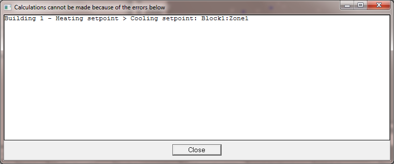
It is important to understand the cause of any errors that occur during an optimisation. The Pause on errors option, when checked, causes a message to be displayed and the optimisation is paused. For example if there is an overlap in heating and cooling setpoint temperatures, in configurations where the heating setpoint is higher than the cooling setpoint the following error message is displayed:
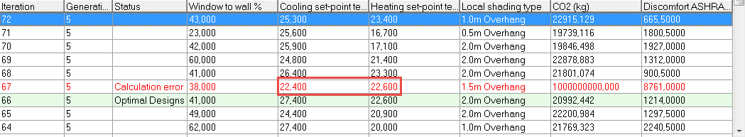
This sort of error does not cause a problem for the overall optimisation study. If a particular design variant has an invalid configuration then it is assigned a penalty using the maximum objective score (assuming objectives are being minimised). This applies evolutionary pressure to discourage similar invalid design variants from appearing in future generations.
Once you are clear about the cause of any errors you will normally want to stop seeing reports and allow the optimisation to continue. To do this simply uncheck the Pause on errors check box. Simulations with errors are displayed in red in the grid as shown below.
Common causes of errors are:
Normally, if DesignBuilder is unable to access the requested Simulation Server, it will ask you whether you would like to Abort, Retry or Ignore the missing server. Selecting Abort cancels the whole analysis. Selecting Retry or Ignore instructs the software to keep trying. The latter option would be selected if the server became temporarily unavailable, perhaps due to a network error or because the server was down for a while.
However, if you are running a long analysis and you don't want to be prompted in this way due to a temporary glitch in the availability of your simulation server then you can check this option. This is similar to pre-selecting the retry or ignore options in advance.
Normally results for each simulation are held within the Simulation Manager system only for as long as required and are deleted once the key results have been loaded into DesignBuilder. However, if you require results for each simulation to be retained within the Simulation Manager system then check this checkbox.
If you are concerned about the stability of the optimisation process (e.g. due to memory issues) you can select this option to ensure that results are stored at the end of each generation, allowing you to later retrieve partially completed results.
An important and often overlooked consideration is the impact of the time taken by DesignBuilder to generate the IDF input file for each design. The longer this is relative to simulation time the greater the model generation bottleneck and the less useful the large number of parallel simulations. On the other hand, the larger and more complex the model and the more detailed the simulations (nat vent, detailed HVAC, more time steps etc) the more time is taken in simulation and relatively less in IDF generation. For an extremely large/complex model, all IDF inputs will have been generated before the first results are in and the large number of parallel simulations will speed progress. For a smaller model, the IDF generation bottleneck is often more significant and first simulation results will be in before the 3rd or 4th IDF input has been generated and in this case the multiple cores will not be used. This is often the case for simple single zone models. To test and understand how this works you may find it useful to watch the standalone Simulation Manager dialog while the optimisation takes place and . You will see new jobs being submitted, queued and simulated.
When 2 objective functions are defined, the trade off for the range of design variables considered is displayed graphically on the scatter graph. The Pareto optimal solutions are displayed in red, current generation are shown in blue and previous generations are shown in dark grey.
When a single objective is used the graphical output shows the evolution of the objective function for each iteration. Because there is no trade off with single objective optimisation, only the single most optimal solution is highlighted in green in the grid.