Performance Curve Coefficient Tools

A range of tools are available to help set up performance curves in a form that can be used in DesignBuilder EnergyPlus simulations based on equipment manufacturers' data sheets:

• DesignBuilder Curve Generator Tool: Accessed from the Info panel of the Curves dialog.

• VRF Curve Generation Utilities: Specialised spreadsheet tools for generating EnergyPlus curves for accurate variable refrigerant flow (VRF) system simulation.

• EnergyPlus Curve Fit Tool: Used to generate HVAC performance curve coefficients for any HVAC equipment modelled with Biquadratic, Cubic, or Quadratic curves using manufacturer data sheets.

• Chiller Performance Curve Coefficients Tool: Used to generate performance curve coefficients for chillers and any other HVAC equipment modelled with Biquadratic, Cubic, or Quadratic curves using manufacturer data sheets.

• Ice Storage Curve Fit Tool: Assists with generating performance curve coefficients for Ice Thermal Storage charge and discharge cycles.
  

All of the above are freely available utilities for generating performance curve coefficients used in HVAC equipment modelling within DesignBuilder/EnergyPlus. They enable users to input performance data at various operating conditions and automatically generate the polynomial coefficients needed to create the curves for accurate equipment simulation. They are commonly used for chillers, heat pumps, DX coils, fans, pumps, and other HVAC equipment.

Notes on the "Chiller Performance Curve Coefficients" and the "EnergyPlus Curve Fit" Tools

 

Both these tools provided by EnergyPlus generate the same curve types (Biquadratic, Cubic, and Quadratic) using identical mathematical principles. Each tool is optimised for its primary workflow, but both offer flexibility for adaptation. Neither tool is strictly limited to a single equipment type or medium (e.g., chillers, heat pumps, air-source vs water-source systems, or water pumps).

 

Both tools are flexible enough to allow you to adapt the independent variable inputs to match your equipment's actual operating conditions. For example, you can adjust the labels and input ranges to represent water temperatures rather than air temperatures, making them suitable for water-to-water systems. See unmet hours article: https://unmethours.com/question/2059/air-source-heat-pump-curves. You can also generate the cubic curves required for water pump part-load performance modelling.

 

Fundamentally, the labels are simply examples tied to the tools' original design intent, while the mathematical curve fitting capability is what makes them generally applicable. Once this principle is clear, you can use either tool (or any other available) for any application requiring Biquadratic, Cubic, or Quadratic curve fitting, regardless of the specific equipment type or operating medium.

For more information on all performance curve types, see: Performance Curve Data.

How DesignBuilder Plots Performance Curves

From the Curves dialog, you can view the performance data as graphical curves on the Curve Plot tab of the dialog.

When DesignBuilder plots a performance curve, the axes and legend representation depends on whether the curve is single-variable or multi-variable:

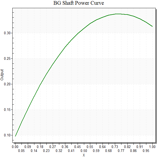
Single-variable curves (e.g., Linear, Quadratic, Cubic, Quartic):

• Horizontal axis (X): The independent variable (e.g., part-load ratio, flow fraction, temperature)

• Vertical axis (Output): The curve's output value (e.g., power modifier, efficiency modifier)

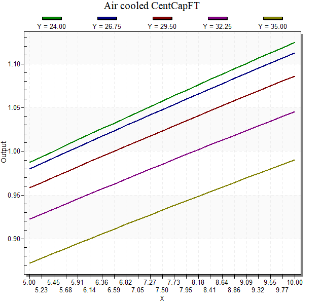
Multi-variable curves (e.g., Biquadratic, Bicubic):

• Horizontal axis (X): The first independent variable (e.g., leaving chilled water temperature)

• Legend entries (Y, colored lines): The second independent variable held constant for each series (e.g., outdoor/source temperature at different fixed values)

• Vertical axis (Output): The curve's output value (e.g., EIR modifier, capacity modifier)

The variable assignment is determined by the order in which you enter your independent variables in the Performance Curve Coefficients tool input table.

For example, when using the DesignBuilder Curve Generator:

• Column x (first variable) → Horizontal axis (X)

• Column y (second variable) → Legend (Y)

Note: Changing the minimum and maximum ranges of X and Y in the Edit Curve will not change which variable is assigned to the horizontal axis or the legend. This only changes the range over which those variables are evaluated.

Example: Chiller EIR Modifier for Temperature Curve (Biquadratic)

For a typical chiller Energy Input Ratio (EIR) modifier curve as a function of two temperatures, consider an example where you have performance data at various leaving chilled water temperatures and entering condenser water temperatures. This section demonstrates both how the plot appears in DesignBuilder and how the coefficient generation is validated across the Curve Generator and Chiller Performance Curve Coefficients tools.

When modelling a chiller's EIR performance, you need to capture how its efficiency changes with:

• First independent variable (x): Supply/Leaving water temperature (CWS)

• Second independent variable (y): Entering condenser water temperature (ECT)

• Value (z) = EIR = 1/COP

EIR modifier as a function of temperature: z = C₁ + C₂ · x + C₃ · x² + C₄ · y + C₅ · y² + C₆ · x · y

You collect performance data at various combinations of these temperatures and enter them into the performance curve tool (e.g., Curve Generator or Chiller_PerformanceCurve_Coefficients) with their corresponding normalised EIR values (relative to rated conditions).

Note: The performance curve tools require that your input data be normalised by dividing the performance value at each condition by the reference/nominal value (e.g., actual EIR / rated EIR). This normalisation is essential because it ensures the resulting curve has a value of 1.0 at reference conditions, which is how DesignBuilder/EnergyPlus interprets the curve during simulation. In Curve Generator this can be done by entering the reference value in the Normalize by field.

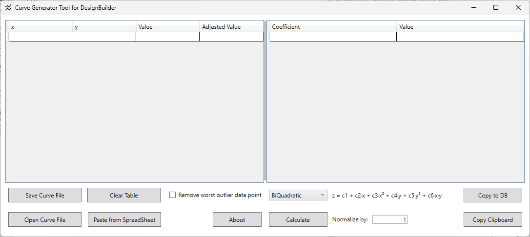
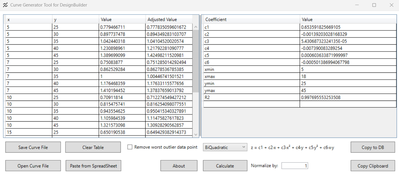
How to Generate Curves Using the Curve Generator

1. Open the Curve Generator tool in DesignBuilder, accessed from the Info panel of the Curves dialog.

2. Select BiQuadratic from the Curve Category dropdown

3. In the input data table, enter:

   • x column: Leaving chilled water temperatures (e.g., 5, 7, 10, 15, 18°C)

   • y column: Entering condenser water temperatures (e.g., 25, 30, 35, 40, 45°C)

   • Value column: Corresponding EIR values at each x, y combination

4. In the Normalize by field, enter the reference EIR value (e.g., if rated COP = 2.71, then reference EIR = 1/2.71 = 0.369)

5. Click on the Calculate button to generate the coefficients

6. The tool in the right panel displays:

   • Six biquadratic coefficients (c1 through c6). These correspond to the biquadratic curve equation:
     z = c1 + c2· x + c3· x² + c4· y + c5· y² + c6· x· y

   • The minimum and maximum x and y values based on the input data range

   • R² value showing goodness-of-fit

7. Click the Copy to DB button to prepare for pasting the coefficients to the DesignBuilder Curve Editor, or Save Curve File for later entry, or Copy to Clipboard to paste the coefficients to a spreadsheet.

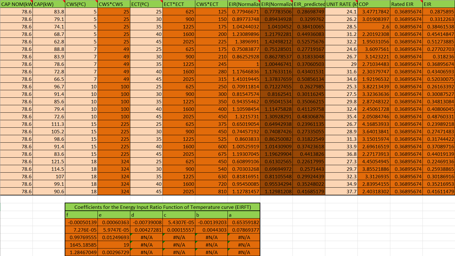
How to Generate Curves Using the Chiller Performance Curve Coefficients Tool

1. Open the Chiller Performance Curve Coefficients spreadsheet tool

2. In the performance data table, enter:

   • CAP_NOM (kW): Rated capacity

   • CAP (kW): Actual capacity at each condition

   • CWS (°C): Leaving chilled water temperatures (e.g., 5, 7, 10, 15, 18°C)

   • ECT (°C): Entering condenser water temperatures (e.g., 25, 30, 35, 40, 45°C)

   • UNIT RATE (kW): Power input

   • Rated EIR: The EIR in nominal conditions

3. The spreadsheet calculates the performance metrics: EIR(Normalized), EIR(Normalized EIR_predicted), COP, and EIR.

4. In the "Coefficients for the Energy Input Ratio Function of Temperature curve (EIRFT)" table, the tool displays:

   • The calculated coefficient values labelled as (a, b, c, d, e, f). These correspond to the standard biquadratic form coefficients in the equation:
     z = a + b · x + c · x² + d · y + e · y² + f · x · y

   • R² value showing goodness-of-fit

   • Other statistical measures from the regression

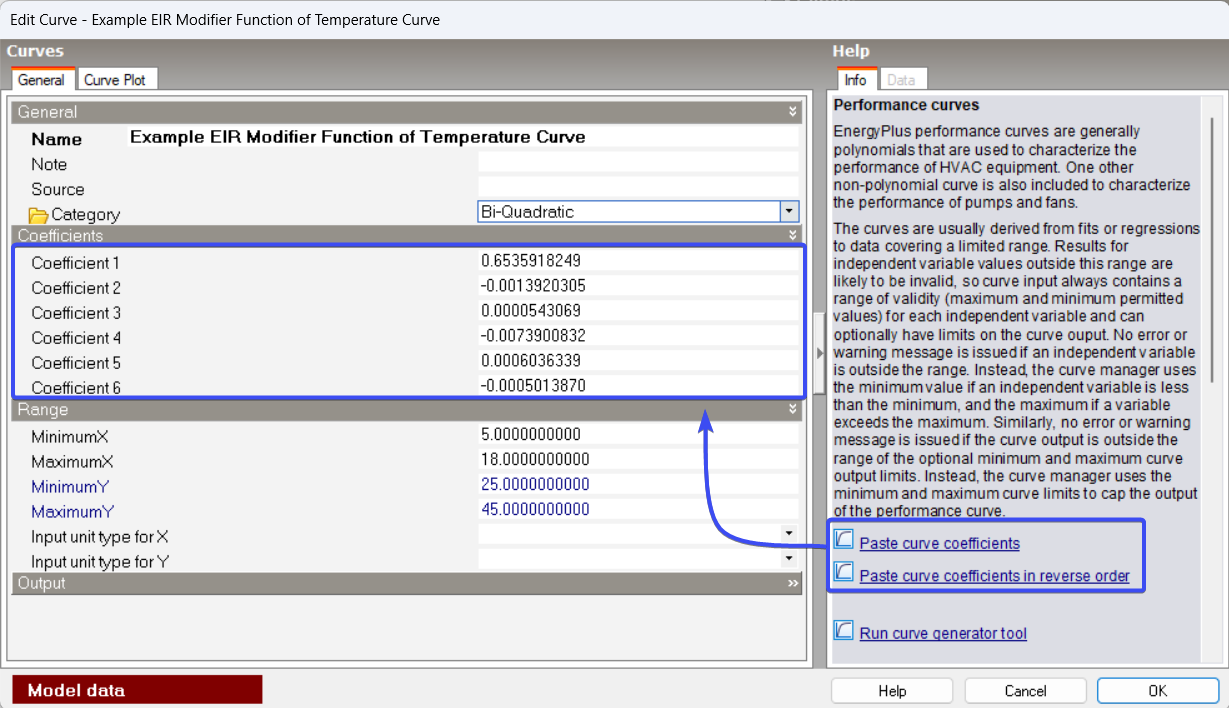
How to Enter Curve Coefficients into DesignBuilder and View the Curve Plot

Once you have generated the coefficients using either tool, you need to enter them into DesignBuilder to use them in your simulation:

1. Navigate to the Detailed HVAC system

2. Select the HVAC component (e.g., Chiller, Plant Loop Heat Pumps)

3. Go to the Performance Curves section

4. Create a copy of an existing Curve or add a new one.

5. Edit the Curve to enter the performance curve coefficients

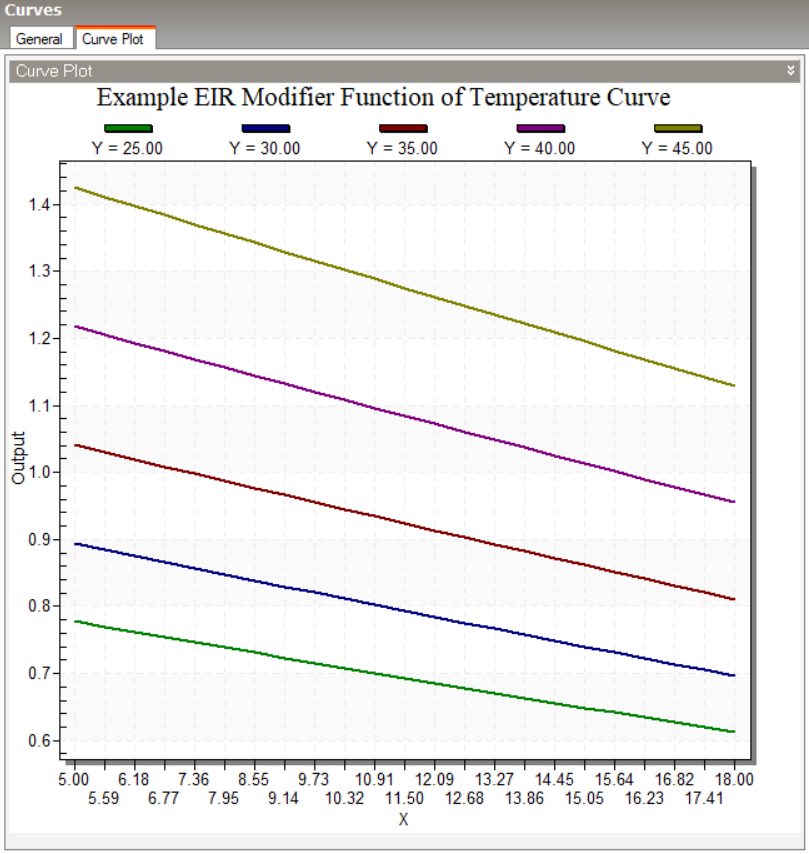
6. Click the Curve Plot tab to visualize the curve

    

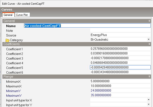
Example "Energy Input Ratio Modifier Function of Temperature Curve":

• Create a copy of an existing Curve or add a new one and name it “Example EIR Modifier Function of Temperature Curve”

• Open the Curve editor

• In the Curve editor choose the appropriate Curve type (e.g., Bi-Quadratic) and enter/paste the coefficients

• Set the curve Range (these should match your xmin, xmax, ymin, ymax values from the Performance Curve Coefficients Tools)

What you will see in the DesignBuilder Curve Plot tab:

• Horizontal axis: Supply water temperatures (e.g., 5°C to 18°C representing leaving water temperature)

• Legend: Outdoor/condenser temperature held constant for each curve (e.g., Y=25, Y=30, Y=35, Y=40, Y=45 representing entering condenser water)

• Vertical axis: The curve output (e.g., EIR modifier value)

Each coloured line shows the multiplier (e.g. EIR multiplier) at different leaving water temperatures while holding the entering condenser water temperature constant. For example, the green line (Y=25°C) shows how EIR varies as leaving chilled water temperature changes from 5°C to 18°C when the condenser temperature is at 25°C.

Important Checks When Using any Performance Curve Coefficients Tool

To ensure accurate curve generation, always verify the following:

1. Column Order and Axis Assignment

    

   Ensure each independent variable in your dataset is mapped to the proper axis. The order of your columns determines which variable appears where on the plot:

    

   • Check that your first independent variable corresponds to what should be on the horizontal axis

   • Check that your second independent variable corresponds to what should be in the legend

   • Refer to DesignBuilder documentation or the EnergyPlus Input/Output Reference to confirm the expected variable order for your specific curve type

      

2. Normalisation Value

    

   Enter the correct reference value to normalise the curve output. Normalisation is essential for ensuring that the curve has a value of 1.0 at reference conditions. This value depends on both the curve type and the equipment being modelled.

   Why this matters: If you enter the wrong normalisation value, your curve will not equal 1.0 at reference conditions, which will cause simulation errors or incorrect equipment performance predictions. DesignBuilder/EnergyPlus uses the curve output of 1.0 at reference conditions as the baseline for scaling equipment performance during simulation. The specific reference value to use (e.g., rated capacity, reference EIR) should be determined based on your equipment data and curve type.

Additional Information

For additional information, refer to the following documentation:

1. Performance Curve Data - General information on performance curves and the Curve Generator tool

2. Heat Pump - Cooling / Heat Pump -Heating - Application of performance curves for heat pumps

3. Chiller:Electric:EIR Technical Description - Detailed technical description of chiller EIR model and its performance curves

4. EnergyPlus Documentation - You can download all the EnergyPlus documentation from here

5. Unmet Hours Article: Determine COP Performance Curves in DesignBuilder for an ASHP - Community discussion on generating and validating heat pump performance curves