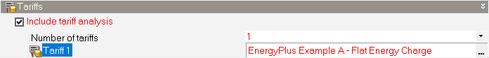
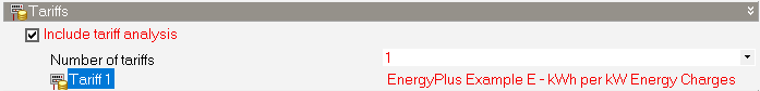
One of the best ways to learn the details of EnergyPlus Economics and how to calculate operational energy costs is to study some example tariffs and how they are entered on the Tariff dialog. The examples below illustrate the process of setting up various tariffs for a range of cases of increasing complexity. Each example includes a description of the tariff to be modelled, step-by-step instructions on how to define it and sample summary output showing the corresponding EnergyPlus economics reports.
Note: The examples provided below are based on entering costs in US Dollars (USD/$), but the principles are the same for all currencies. The Currency can be selected on the International tab of the Program options dialog.
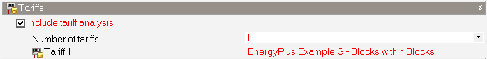
The tariffs described below under Examples A-J headings can be set up for any model. However, if you would like to reproduce the summary results provided to aid your learning process, you should apply the tariffs to the same base model used to create the results below. You can create the base model by following the steps below.
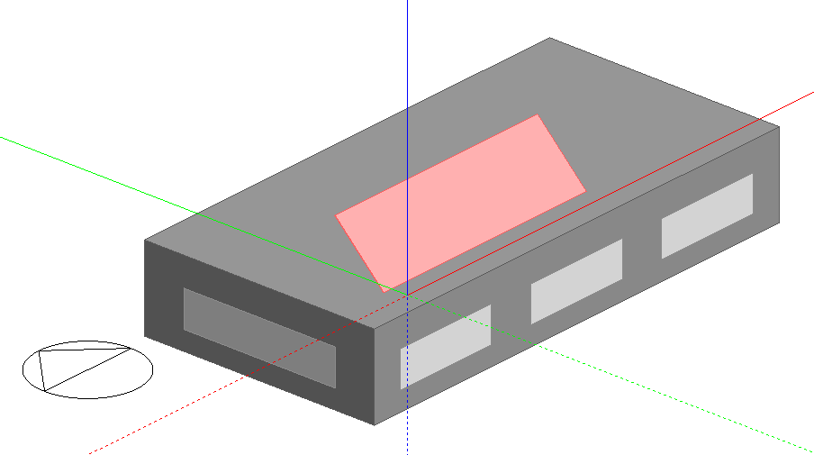
1. Create a new file located in London Gatwick and add a building to the site with a simple rectangular block having dimensions 20m x 10m as shown below. Start by using default Model options and template settings.
2. Set the Detailed HVAC model option. This is a required step as EnergyPlus Economics only works with full HVAC system definitions.
3. Load the default "FCU 4-pipe, Air-cooled Chiller" Detailed HVAC template.
4. Add a PV panel on the roof with dimensions 10m x 3m and rotate it so it faces south with an inclination of 45°.
5. Connect the PV panel to a distribution centre. To do this, go to the Generation tab, create a new Load centre by copying the existing default "DC with Inverter" library load centre. On the Generator List tab, select your Solar collector.
The PV panel will be used in Example I to illustrate "net metering" and cases where electricity is sold back to the utility.
The model should now look similar to the screenshot below.
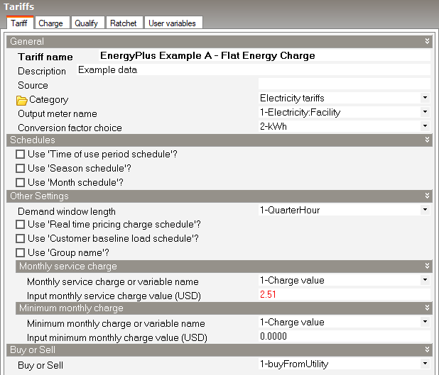
This example shows how to define a simple tariff which charges for electricity at a constant rate with a fixed monthly service fee. This simple approach is suitable for utilities or contracts that charge a flat rate without tiered pricing or demand charges.
Customer charge: $2.51 per month
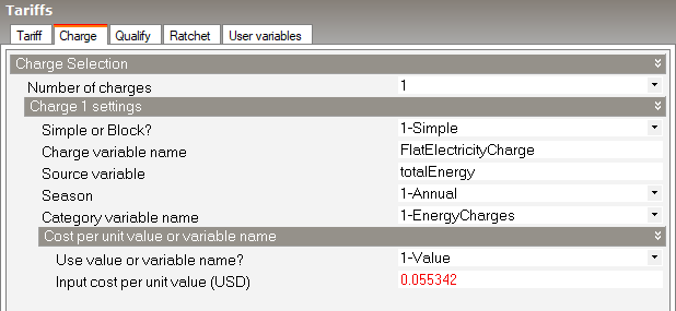
Energy charge: 5.5342 cents/kWh
This simple tariff can be set up by making the following settings on the Economics tab at building level.
To create this tariff structure, follow the steps below.
1. Create a new Tariff component:
2. On the Tariff tab of the Tariff dialog, set the fixed monthly fee to $2.51 per month using the Input monthly service charge value setting as shown below:
3. On the Charge tab:
Set the Number of charges to 1.
Under the Charge 1 settings header:
Set Simple or Block? to 1-Simple.
Set the Input cost per unit value to 0.055342 USD:
Report: Economics Results Summary Report
For: Entire Facility
Timestamp: 2025-09-11 11:48:03
Annual Cost
| Electricity | Natural Gas | Other | Total | |
| Cost [$] | 979.83 | 0.00 | 0.00 | 979.83 |
| Cost per Total Building Area [$/m2] | 5.36 | 0.00 | 0.00 | 5.36 |
| Cost per Net Conditioned Building Area [$/m2] | 5.36 | 0.00 | 0.00 | 5.36 |
Tariff Summary
| Selected | Qualified | Meter | Buy or Sell | Group | Annual Cost ($) | |
| ENERGYPLUS EXAMPLE A - FLAT ENERGY CHARGE | Yes | Yes | ELECTRICITY:FACILITY | Buy | (none) | 979.83 |
Report: Tariff Report
For: ENERGYPLUS EXAMPLE A - FLAT ENERGY CHARGE
Timestamp: 2025-09-11 11:48:03
General
| Parameter | |
| Meter | ELECTRICITY:FACILITY |
| Selected | Yes |
| Group | (none) |
| Qualified | Yes |
| Disqualifier | n/a |
| Computation | automatic |
| Units | kWh |
Categories
| Jan | Feb | Mar | Apr | May | Jun | Jul | Aug | Sep | Oct | Nov | Dec | Sum | Max | |
| EnergyCharges ($) | 69.77 | 61.62 | 67.12 | 79.32 | 93.67 | 84.19 | 102.31 | 95.69 | 83.57 | 79.81 | 65.45 | 67.20 | 949.71 | 102.31 |
| DemandCharges ($) | 0.00 | 0.00 | 0.00 | 0.00 | 0.00 | 0.00 | 0.00 | 0.00 | 0.00 | 0.00 | 0.00 | 0.00 | 0.00 | 0.00 |
| ServiceCharges ($) | 2.51 | 2.51 | 2.51 | 2.51 | 2.51 | 2.51 | 2.51 | 2.51 | 2.51 | 2.51 | 2.51 | 2.51 | 30.12 | 2.51 |
| Basis ($) | 72.28 | 64.13 | 69.63 | 81.83 | 96.18 | 86.70 | 104.82 | 98.20 | 86.08 | 82.32 | 67.96 | 69.71 | 979.83 | 104.82 |
| Adjustment ($) | 0.00 | 0.00 | 0.00 | 0.00 | 0.00 | 0.00 | 0.00 | 0.00 | 0.00 | 0.00 | 0.00 | 0.00 | 0.00 | 0.00 |
| Surcharge ($) | 0.00 | 0.00 | 0.00 | 0.00 | 0.00 | 0.00 | 0.00 | 0.00 | 0.00 | 0.00 | 0.00 | 0.00 | 0.00 | 0.00 |
| Subtotal ($) | 72.28 | 64.13 | 69.63 | 81.83 | 96.18 | 86.70 | 104.82 | 98.20 | 86.08 | 82.32 | 67.96 | 69.71 | 979.83 | 104.82 |
| Taxes ($) | 0.00 | 0.00 | 0.00 | 0.00 | 0.00 | 0.00 | 0.00 | 0.00 | 0.00 | 0.00 | 0.00 | 0.00 | 0.00 | 0.00 |
| Total ($) | 72.28 | 64.13 | 69.63 | 81.83 | 96.18 | 86.70 | 104.82 | 98.20 | 86.08 | 82.32 | 67.96 | 69.71 | 979.83 | 104.82 |
Charges
| Jan | Feb | Mar | Apr | May | Jun | Jul | Aug | Sep | Oct | Nov | Dec | Sum | Max | Category | |
| FLATELECTRICITYCHARGE ($) | 69.77 | 61.62 | 67.12 | 79.32 | 93.67 | 84.19 | 102.31 | 95.69 | 83.57 | 79.81 | 65.45 | 67.20 | 949.71 | 102.31 | EnergyCharges |
Corresponding Sources for Charges
| Jan | Feb | Mar | Apr | May | Jun | Jul | Aug | Sep | Oct | Nov | Dec | Sum | Max | |
| TotalEnergy | 1260.67 | 1113.39 | 1212.74 | 1433.24 | 1692.60 | 1521.19 | 1848.65 | 1729.11 | 1510.12 | 1442.16 | 1182.59 | 1214.35 | 17160.81 | 1848.65 |
Ratchets
| Jan | Feb | Mar | Apr | May | Jun | Jul | Aug | Sep | Oct | Nov | Dec | Sum | Max |
Qualifies
| Jan | Feb | Mar | Apr | May | Jun | Jul | Aug | Sep | Oct | Nov | Dec | Sum | Max |
Native Variables
| Jan | Feb | Mar | Apr | May | Jun | Jul | Aug | Sep | Oct | Nov | Dec | Sum | Max | |
| TotalEnergy | 1260.67 | 1113.39 | 1212.74 | 1433.24 | 1692.60 | 1521.19 | 1848.65 | 1729.11 | 1510.12 | 1442.16 | 1182.59 | 1214.35 | 17160.81 | 1848.65 |
| TotalDemand | 4.07 | 5.44 | 5.82 | 6.15 | 6.75 | 7.53 | 7.60 | 7.94 | 6.66 | 6.12 | 5.64 | 4.07 | 73.78 | 7.94 |
| PeakEnergy | 1260.67 | 1113.39 | 1212.74 | 1433.24 | 1692.60 | 1521.19 | 1848.65 | 1729.11 | 1510.12 | 1442.16 | 1182.59 | 1214.35 | 17160.81 | 1848.65 |
| PeakDemand | 4.07 | 5.44 | 5.82 | 6.15 | 6.75 | 7.53 | 7.60 | 7.94 | 6.66 | 6.12 | 5.64 | 4.07 | 73.78 | 7.94 |
| ShoulderEnergy | 0.00 | 0.00 | 0.00 | 0.00 | 0.00 | 0.00 | 0.00 | 0.00 | 0.00 | 0.00 | 0.00 | 0.00 | 0.00 | 0.00 |
| ShoulderDemand | 0.00 | 0.00 | 0.00 | 0.00 | 0.00 | 0.00 | 0.00 | 0.00 | 0.00 | 0.00 | 0.00 | 0.00 | 0.00 | 0.00 |
| OffPeakEnergy | 0.00 | 0.00 | 0.00 | 0.00 | 0.00 | 0.00 | 0.00 | 0.00 | 0.00 | 0.00 | 0.00 | 0.00 | 0.00 | 0.00 |
| OffPeakDemand | 0.00 | 0.00 | 0.00 | 0.00 | 0.00 | 0.00 | 0.00 | 0.00 | 0.00 | 0.00 | 0.00 | 0.00 | 0.00 | 0.00 |
| MidPeakEnergy | 0.00 | 0.00 | 0.00 | 0.00 | 0.00 | 0.00 | 0.00 | 0.00 | 0.00 | 0.00 | 0.00 | 0.00 | 0.00 | 0.00 |
| MidPeakDemand | 0.00 | 0.00 | 0.00 | 0.00 | 0.00 | 0.00 | 0.00 | 0.00 | 0.00 | 0.00 | 0.00 | 0.00 | 0.00 | 0.00 |
| PeakExceedsOffPeak | 4.07 | 5.44 | 5.82 | 6.15 | 6.75 | 7.53 | 7.60 | 7.94 | 6.66 | 6.12 | 5.64 | 4.07 | 73.78 | 7.94 |
| OffPeakExceedsPeak | 0.00 | 0.00 | 0.00 | 0.00 | 0.00 | 0.00 | 0.00 | 0.00 | 0.00 | 0.00 | 0.00 | 0.00 | 0.00 | 0.00 |
| PeakExceedsMidPeak | 4.07 | 5.44 | 5.82 | 6.15 | 6.75 | 7.53 | 7.60 | 7.94 | 6.66 | 6.12 | 5.64 | 4.07 | 73.78 | 7.94 |
| MidPeakExceedsPeak | 0.00 | 0.00 | 0.00 | 0.00 | 0.00 | 0.00 | 0.00 | 0.00 | 0.00 | 0.00 | 0.00 | 0.00 | 0.00 | 0.00 |
| PeakExceedsShoulder | 4.07 | 5.44 | 5.82 | 6.15 | 6.75 | 7.53 | 7.60 | 7.94 | 6.66 | 6.12 | 5.64 | 4.07 | 73.78 | 7.94 |
| ShoulderExceedsPeak | 0.00 | 0.00 | 0.00 | 0.00 | 0.00 | 0.00 | 0.00 | 0.00 | 0.00 | 0.00 | 0.00 | 0.00 | 0.00 | 0.00 |
| IsWinter | 1.00 | 1.00 | 1.00 | 1.00 | 1.00 | 1.00 | 1.00 | 1.00 | 1.00 | 1.00 | 1.00 | 1.00 | 12.00 | 1.00 |
| IsNotWinter | 0.00 | 0.00 | 0.00 | 0.00 | 0.00 | 0.00 | 0.00 | 0.00 | 0.00 | 0.00 | 0.00 | 0.00 | 0.00 | 0.00 |
| IsSpring | 0.00 | 0.00 | 0.00 | 0.00 | 0.00 | 0.00 | 0.00 | 0.00 | 0.00 | 0.00 | 0.00 | 0.00 | 0.00 | 0.00 |
| IsNotSpring | 1.00 | 1.00 | 1.00 | 1.00 | 1.00 | 1.00 | 1.00 | 1.00 | 1.00 | 1.00 | 1.00 | 1.00 | 12.00 | 1.00 |
| IsSummer | 0.00 | 0.00 | 0.00 | 0.00 | 0.00 | 0.00 | 0.00 | 0.00 | 0.00 | 0.00 | 0.00 | 0.00 | 0.00 | 0.00 |
| IsNotSummer | 1.00 | 1.00 | 1.00 | 1.00 | 1.00 | 1.00 | 1.00 | 1.00 | 1.00 | 1.00 | 1.00 | 1.00 | 12.00 | 1.00 |
| IsAutumn | 0.00 | 0.00 | 0.00 | 0.00 | 0.00 | 0.00 | 0.00 | 0.00 | 0.00 | 0.00 | 0.00 | 0.00 | 0.00 | 0.00 |
| IsNotAutumn | 1.00 | 1.00 | 1.00 | 1.00 | 1.00 | 1.00 | 1.00 | 1.00 | 1.00 | 1.00 | 1.00 | 1.00 | 12.00 | 1.00 |
| PeakAndShoulderEnergy | 1260.67 | 1113.39 | 1212.74 | 1433.24 | 1692.60 | 1521.19 | 1848.65 | 1729.11 | 1510.12 | 1442.16 | 1182.59 | 1214.35 | 17160.81 | 1848.65 |
| PeakAndShoulderDemand | 4.07 | 5.44 | 5.82 | 6.15 | 6.75 | 7.53 | 7.60 | 7.94 | 6.66 | 6.12 | 5.64 | 4.07 | 73.78 | 7.94 |
| PeakAndMidPeakEnergy | 1260.67 | 1113.39 | 1212.74 | 1433.24 | 1692.60 | 1521.19 | 1848.65 | 1729.11 | 1510.12 | 1442.16 | 1182.59 | 1214.35 | 17160.81 | 1848.65 |
| PeakAndMidPeakDemand | 4.07 | 5.44 | 5.82 | 6.15 | 6.75 | 7.53 | 7.60 | 7.94 | 6.66 | 6.12 | 5.64 | 4.07 | 73.78 | 7.94 |
| ShoulderAndOffPeakEnergy | 0.00 | 0.00 | 0.00 | 0.00 | 0.00 | 0.00 | 0.00 | 0.00 | 0.00 | 0.00 | 0.00 | 0.00 | 0.00 | 0.00 |
| ShoulderAndOffPeakDemand | 0.00 | 0.00 | 0.00 | 0.00 | 0.00 | 0.00 | 0.00 | 0.00 | 0.00 | 0.00 | 0.00 | 0.00 | 0.00 | 0.00 |
| PeakAndOffPeakEnergy | 1260.67 | 1113.39 | 1212.74 | 1433.24 | 1692.60 | 1521.19 | 1848.65 | 1729.11 | 1510.12 | 1442.16 | 1182.59 | 1214.35 | 17160.81 | 1848.65 |
| PeakAndOffPeakDemand | 4.07 | 5.44 | 5.82 | 6.15 | 6.75 | 7.53 | 7.60 | 7.94 | 6.66 | 6.12 | 5.64 | 4.07 | 73.78 | 7.94 |
| RealTimePriceCosts | 0.00 | 0.00 | 0.00 | 0.00 | 0.00 | 0.00 | 0.00 | 0.00 | 0.00 | 0.00 | 0.00 | 0.00 | 0.00 | 0.00 |
| AboveCustomerBaseCosts | 0.00 | 0.00 | 0.00 | 0.00 | 0.00 | 0.00 | 0.00 | 0.00 | 0.00 | 0.00 | 0.00 | 0.00 | 0.00 | 0.00 |
| BelowCustomerBaseCosts | 0.00 | 0.00 | 0.00 | 0.00 | 0.00 | 0.00 | 0.00 | 0.00 | 0.00 | 0.00 | 0.00 | 0.00 | 0.00 | 0.00 |
| AboveCustomerBaseEnergy | 0.00 | 0.00 | 0.00 | 0.00 | 0.00 | 0.00 | 0.00 | 0.00 | 0.00 | 0.00 | 0.00 | 0.00 | 0.00 | 0.00 |
| BelowCustomerBaseEnergy | 0.00 | 0.00 | 0.00 | 0.00 | 0.00 | 0.00 | 0.00 | 0.00 | 0.00 | 0.00 | 0.00 | 0.00 | 0.00 | 0.00 |
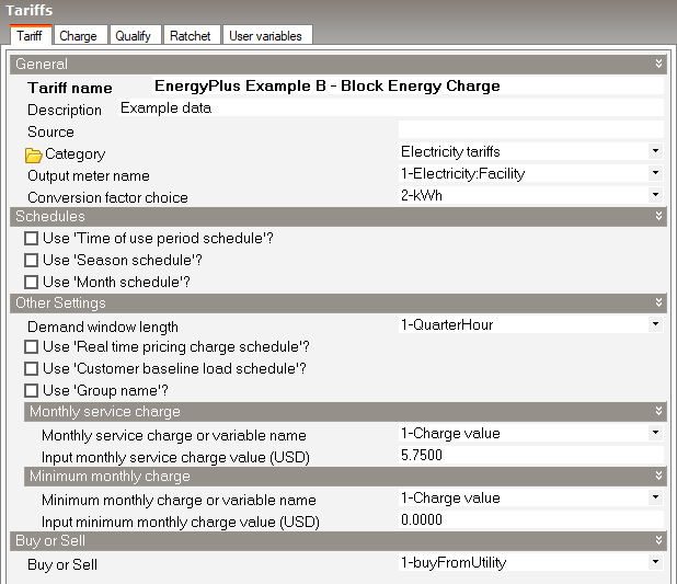
This example adds tiered energy pricing blocks to a flat fee, where cost decreases as consumption increases. This is common for residential or small commercial tariffs with step-down pricing to make higher usage rates more affordable.
Customer charge: $5.75 per month
Energy charges:
7.231 cents/kWh for first 200 kWh
6.656 cents/kWh for next 1000 kWh
5.876 cents/kWh for over 1200 kWh
To create this tariff structure, follow the steps below.
1. Create a new Tariff component:
2. On the Tariff tab of the Tariff dialog:
Set the fixed monthly fee to $5.75 per month using the Input monthly service charge value setting as shown below:
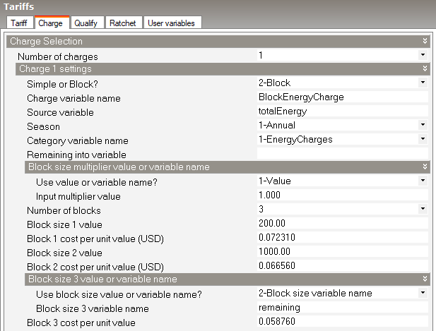
3. On the Charge tab:
Set the Number of charges to 1.
Under the Charge 1 settings header:
Set Simple or Block? to 2-Block
Set Source variable to totalEnergy
Set the Number of blocks to 3
Set Block size 1 value to 200.
Set Block 1 cost per unit value to 0.07231 USD.
Set Block size 2 value to 1000.
Set the Block 2 cost per unit value to 0.06656 USD.
Set the Block size 3 variable name to remaining.
Set the Block 3 cost per unit value to 0.05876 USD.
The screenshot below show how the charge tab should look when you have finished.
Report: Economics Results Summary Report
For: Entire Facility
Timestamp: 2025-09-11 11:44:35
Annual Cost
| Electricity | Natural Gas | Other | Total | |
| Cost [$] | 1202.68 | 0.00 | 0.00 | 1202.68 |
| Cost per Total Building Area [$/m2] | 6.58 | 0.00 | 0.00 | 6.58 |
| Cost per Net Conditioned Building Area [$/m2] | 6.58 | 0.00 | 0.00 | 6.58 |
Tariff Summary
| Selected | Qualified | Meter | Buy or Sell | Group | Annual Cost ($) | |
| ENERGYPLUS EXAMPLE B - BLOCK ENERGY CHARGE | Yes | Yes | ELECTRICITY:FACILITY | Buy | (none) | 1202.68 |
Report: Tariff Report
For: ENERGYPLUS EXAMPLE B - BLOCK ENERGY CHARGE
Timestamp: 2025-09-11 11:44:35
General
| Parameter | |
| Meter | ELECTRICITY:FACILITY |
| Selected | Yes |
| Group | (none) |
| Qualified | Yes |
| Disqualifier | n/a |
| Computation | automatic |
| Units | kWh |
Categories
| Jan | Feb | Mar | Apr | May | Jun | Jul | Aug | Sep | Oct | Nov | Dec | Sum | Max | |
| EnergyCharges ($) | 84.59 | 75.26 | 81.77 | 94.73 | 109.97 | 99.90 | 119.14 | 112.11 | 99.24 | 95.25 | 79.86 | 81.87 | 1133.68 | 119.14 |
| DemandCharges ($) | 0.00 | 0.00 | 0.00 | 0.00 | 0.00 | 0.00 | 0.00 | 0.00 | 0.00 | 0.00 | 0.00 | 0.00 | 0.00 | 0.00 |
| ServiceCharges ($) | 5.75 | 5.75 | 5.75 | 5.75 | 5.75 | 5.75 | 5.75 | 5.75 | 5.75 | 5.75 | 5.75 | 5.75 | 69.00 | 5.75 |
| Basis ($) | 90.34 | 81.01 | 87.52 | 100.48 | 115.72 | 105.65 | 124.89 | 117.86 | 104.99 | 101.00 | 85.61 | 87.62 | 1202.68 | 124.89 |
| Adjustment ($) | 0.00 | 0.00 | 0.00 | 0.00 | 0.00 | 0.00 | 0.00 | 0.00 | 0.00 | 0.00 | 0.00 | 0.00 | 0.00 | 0.00 |
| Surcharge ($) | 0.00 | 0.00 | 0.00 | 0.00 | 0.00 | 0.00 | 0.00 | 0.00 | 0.00 | 0.00 | 0.00 | 0.00 | 0.00 | 0.00 |
| Subtotal ($) | 90.34 | 81.01 | 87.52 | 100.48 | 115.72 | 105.65 | 124.89 | 117.86 | 104.99 | 101.00 | 85.61 | 87.62 | 1202.68 | 124.89 |
| Taxes ($) | 0.00 | 0.00 | 0.00 | 0.00 | 0.00 | 0.00 | 0.00 | 0.00 | 0.00 | 0.00 | 0.00 | 0.00 | 0.00 | 0.00 |
| Total ($) | 90.34 | 81.01 | 87.52 | 100.48 | 115.72 | 105.65 | 124.89 | 117.86 | 104.99 | 101.00 | 85.61 | 87.62 | 1202.68 | 124.89 |
Charges
| Jan | Feb | Mar | Apr | May | Jun | Jul | Aug | Sep | Oct | Nov | Dec | Sum | Max | Category | |
| BLOCKENERGYCHARGE ($) | 84.59 | 75.26 | 81.77 | 94.73 | 109.97 | 99.90 | 119.14 | 112.11 | 99.24 | 95.25 | 79.86 | 81.87 | 1133.68 | 119.14 | EnergyCharges |
Corresponding Sources for Charges
| Jan | Feb | Mar | Apr | May | Jun | Jul | Aug | Sep | Oct | Nov | Dec | Sum | Max | |
| TotalEnergy | 1260.67 | 1113.39 | 1212.74 | 1433.24 | 1692.60 | 1521.19 | 1848.65 | 1729.11 | 1510.12 | 1442.16 | 1182.59 | 1214.35 | 17160.81 | 1848.65 |
Ratchets
| Jan | Feb | Mar | Apr | May | Jun | Jul | Aug | Sep | Oct | Nov | Dec | Sum | Max |
Qualifies
| Jan | Feb | Mar | Apr | May | Jun | Jul | Aug | Sep | Oct | Nov | Dec | Sum | Max |
Native Variables
| Jan | Feb | Mar | Apr | May | Jun | Jul | Aug | Sep | Oct | Nov | Dec | Sum | Max | |
| TotalEnergy | 1260.67 | 1113.39 | 1212.74 | 1433.24 | 1692.60 | 1521.19 | 1848.65 | 1729.11 | 1510.12 | 1442.16 | 1182.59 | 1214.35 | 17160.81 | 1848.65 |
| TotalDemand | 4.07 | 5.44 | 5.82 | 6.15 | 6.75 | 7.53 | 7.60 | 7.94 | 6.66 | 6.12 | 5.64 | 4.07 | 73.78 | 7.94 |
| PeakEnergy | 1260.67 | 1113.39 | 1212.74 | 1433.24 | 1692.60 | 1521.19 | 1848.65 | 1729.11 | 1510.12 | 1442.16 | 1182.59 | 1214.35 | 17160.81 | 1848.65 |
| PeakDemand | 4.07 | 5.44 | 5.82 | 6.15 | 6.75 | 7.53 | 7.60 | 7.94 | 6.66 | 6.12 | 5.64 | 4.07 | 73.78 | 7.94 |
| ShoulderEnergy | 0.00 | 0.00 | 0.00 | 0.00 | 0.00 | 0.00 | 0.00 | 0.00 | 0.00 | 0.00 | 0.00 | 0.00 | 0.00 | 0.00 |
| ShoulderDemand | 0.00 | 0.00 | 0.00 | 0.00 | 0.00 | 0.00 | 0.00 | 0.00 | 0.00 | 0.00 | 0.00 | 0.00 | 0.00 | 0.00 |
| OffPeakEnergy | 0.00 | 0.00 | 0.00 | 0.00 | 0.00 | 0.00 | 0.00 | 0.00 | 0.00 | 0.00 | 0.00 | 0.00 | 0.00 | 0.00 |
| OffPeakDemand | 0.00 | 0.00 | 0.00 | 0.00 | 0.00 | 0.00 | 0.00 | 0.00 | 0.00 | 0.00 | 0.00 | 0.00 | 0.00 | 0.00 |
| MidPeakEnergy | 0.00 | 0.00 | 0.00 | 0.00 | 0.00 | 0.00 | 0.00 | 0.00 | 0.00 | 0.00 | 0.00 | 0.00 | 0.00 | 0.00 |
| MidPeakDemand | 0.00 | 0.00 | 0.00 | 0.00 | 0.00 | 0.00 | 0.00 | 0.00 | 0.00 | 0.00 | 0.00 | 0.00 | 0.00 | 0.00 |
| PeakExceedsOffPeak | 4.07 | 5.44 | 5.82 | 6.15 | 6.75 | 7.53 | 7.60 | 7.94 | 6.66 | 6.12 | 5.64 | 4.07 | 73.78 | 7.94 |
| OffPeakExceedsPeak | 0.00 | 0.00 | 0.00 | 0.00 | 0.00 | 0.00 | 0.00 | 0.00 | 0.00 | 0.00 | 0.00 | 0.00 | 0.00 | 0.00 |
| PeakExceedsMidPeak | 4.07 | 5.44 | 5.82 | 6.15 | 6.75 | 7.53 | 7.60 | 7.94 | 6.66 | 6.12 | 5.64 | 4.07 | 73.78 | 7.94 |
| MidPeakExceedsPeak | 0.00 | 0.00 | 0.00 | 0.00 | 0.00 | 0.00 | 0.00 | 0.00 | 0.00 | 0.00 | 0.00 | 0.00 | 0.00 | 0.00 |
| PeakExceedsShoulder | 4.07 | 5.44 | 5.82 | 6.15 | 6.75 | 7.53 | 7.60 | 7.94 | 6.66 | 6.12 | 5.64 | 4.07 | 73.78 | 7.94 |
| ShoulderExceedsPeak | 0.00 | 0.00 | 0.00 | 0.00 | 0.00 | 0.00 | 0.00 | 0.00 | 0.00 | 0.00 | 0.00 | 0.00 | 0.00 | 0.00 |
| IsWinter | 1.00 | 1.00 | 1.00 | 1.00 | 1.00 | 1.00 | 1.00 | 1.00 | 1.00 | 1.00 | 1.00 | 1.00 | 12.00 | 1.00 |
| IsNotWinter | 0.00 | 0.00 | 0.00 | 0.00 | 0.00 | 0.00 | 0.00 | 0.00 | 0.00 | 0.00 | 0.00 | 0.00 | 0.00 | 0.00 |
| IsSpring | 0.00 | 0.00 | 0.00 | 0.00 | 0.00 | 0.00 | 0.00 | 0.00 | 0.00 | 0.00 | 0.00 | 0.00 | 0.00 | 0.00 |
| IsNotSpring | 1.00 | 1.00 | 1.00 | 1.00 | 1.00 | 1.00 | 1.00 | 1.00 | 1.00 | 1.00 | 1.00 | 1.00 | 12.00 | 1.00 |
| IsSummer | 0.00 | 0.00 | 0.00 | 0.00 | 0.00 | 0.00 | 0.00 | 0.00 | 0.00 | 0.00 | 0.00 | 0.00 | 0.00 | 0.00 |
| IsNotSummer | 1.00 | 1.00 | 1.00 | 1.00 | 1.00 | 1.00 | 1.00 | 1.00 | 1.00 | 1.00 | 1.00 | 1.00 | 12.00 | 1.00 |
| IsAutumn | 0.00 | 0.00 | 0.00 | 0.00 | 0.00 | 0.00 | 0.00 | 0.00 | 0.00 | 0.00 | 0.00 | 0.00 | 0.00 | 0.00 |
| IsNotAutumn | 1.00 | 1.00 | 1.00 | 1.00 | 1.00 | 1.00 | 1.00 | 1.00 | 1.00 | 1.00 | 1.00 | 1.00 | 12.00 | 1.00 |
| PeakAndShoulderEnergy | 1260.67 | 1113.39 | 1212.74 | 1433.24 | 1692.60 | 1521.19 | 1848.65 | 1729.11 | 1510.12 | 1442.16 | 1182.59 | 1214.35 | 17160.81 | 1848.65 |
| PeakAndShoulderDemand | 4.07 | 5.44 | 5.82 | 6.15 | 6.75 | 7.53 | 7.60 | 7.94 | 6.66 | 6.12 | 5.64 | 4.07 | 73.78 | 7.94 |
| PeakAndMidPeakEnergy | 1260.67 | 1113.39 | 1212.74 | 1433.24 | 1692.60 | 1521.19 | 1848.65 | 1729.11 | 1510.12 | 1442.16 | 1182.59 | 1214.35 | 17160.81 | 1848.65 |
| PeakAndMidPeakDemand | 4.07 | 5.44 | 5.82 | 6.15 | 6.75 | 7.53 | 7.60 | 7.94 | 6.66 | 6.12 | 5.64 | 4.07 | 73.78 | 7.94 |
| ShoulderAndOffPeakEnergy | 0.00 | 0.00 | 0.00 | 0.00 | 0.00 | 0.00 | 0.00 | 0.00 | 0.00 | 0.00 | 0.00 | 0.00 | 0.00 | 0.00 |
| ShoulderAndOffPeakDemand | 0.00 | 0.00 | 0.00 | 0.00 | 0.00 | 0.00 | 0.00 | 0.00 | 0.00 | 0.00 | 0.00 | 0.00 | 0.00 | 0.00 |
| PeakAndOffPeakEnergy | 1260.67 | 1113.39 | 1212.74 | 1433.24 | 1692.60 | 1521.19 | 1848.65 | 1729.11 | 1510.12 | 1442.16 | 1182.59 | 1214.35 | 17160.81 | 1848.65 |
| PeakAndOffPeakDemand | 4.07 | 5.44 | 5.82 | 6.15 | 6.75 | 7.53 | 7.60 | 7.94 | 6.66 | 6.12 | 5.64 | 4.07 | 73.78 | 7.94 |
| RealTimePriceCosts | 0.00 | 0.00 | 0.00 | 0.00 | 0.00 | 0.00 | 0.00 | 0.00 | 0.00 | 0.00 | 0.00 | 0.00 | 0.00 | 0.00 |
| AboveCustomerBaseCosts | 0.00 | 0.00 | 0.00 | 0.00 | 0.00 | 0.00 | 0.00 | 0.00 | 0.00 | 0.00 | 0.00 | 0.00 | 0.00 | 0.00 |
| BelowCustomerBaseCosts | 0.00 | 0.00 | 0.00 | 0.00 | 0.00 | 0.00 | 0.00 | 0.00 | 0.00 | 0.00 | 0.00 | 0.00 | 0.00 | 0.00 |
| AboveCustomerBaseEnergy | 0.00 | 0.00 | 0.00 | 0.00 | 0.00 | 0.00 | 0.00 | 0.00 | 0.00 | 0.00 | 0.00 | 0.00 | 0.00 | 0.00 |
| BelowCustomerBaseEnergy | 0.00 | 0.00 | 0.00 | 0.00 | 0.00 | 0.00 | 0.00 | 0.00 | 0.00 | 0.00 | 0.00 | 0.00 | 0.00 | 0.00 |
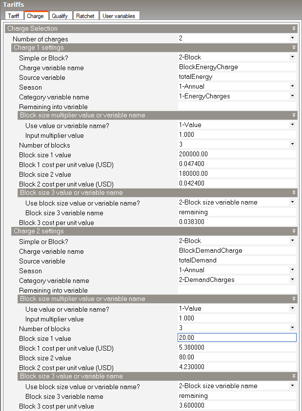
This example uses separate block structures for energy and demand charges. This approach is suitable for modelling commercial tariffs that include both consumption and peak demand billing components. Demand charges encourage customers to manage their peak usage patterns, not just total consumption. It is similar to the previous example except it includes demand charges as well. The energy and demand charges vary by the amount of energy and demand consumed each month.
Energy charges:
4.74 cents/kWh for first 20,000 kWh
4.24 cents/kWh for next 180,000 kWh
3.83 cents/kWh for additional kWh
Demand charges:
5.38 dollars per kW for first 20 kW
4.23 dollars per kW for next 80 kW
3.60 dollars per kW for additional kW
To create this tariff structure, follow the steps below.
1. Create a new Tariff component:
2. On the Tariff tab of the Tariff dialog, clear any fixed tariff data as shown below:
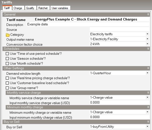
3. On the Charge tab:
Set the Number of charges to 2, the first covering energy, the other for demand.
Under the Charge 1 settings header:
Set Simple or Block? to 2-Block.
Set Charge variable name to BlockEnergyCharge
Set Source variable to totalEnergy
Set the Number of blocks to 3
Set Block size 1 value to 20,000.
Set Block 1 cost per unit value to 0.0474 USD.
Set Block size 2 value to 180,000.
Set the Block 2 cost per unit value to 0.0424 USD.
Set the Block size 3 variable name to remaining.
Set the Block 3 cost per unit value to 0.0383 USD.
Under the Charge 2 settings header:
Set Simple or Block? to 2-Block.
Set Charge variable name to BlockDemandCharge
Set Source variable to totalDemand
Set Category variable name to 2-DemandCharges
Set the Number of blocks to 3
Set Block size 1 value to 20.
Set Block 1 cost per unit value to 5.38 USD.
Set Block size 2 value to 80.
Set the Block 2 cost per unit value to 4.23 USD.
Set the Block size 3 variable name to remaining.
Set the Block 3 cost per unit value to 3.60 USD.
The screenshot below show how the charge tab should look when you have finished.
Report: Economics Results Summary Report
For: Entire Facility
Timestamp: 2025-09-15 11:11:40
Annual Cost
| Electricity | Natural Gas | Other | Total | |
| Cost [$] | 1211.76 | 0.00 | 0.00 | 1211.76 |
| Cost per Total Building Area [$/m2] | 6.63 | 0.00 | 0.00 | 6.63 |
| Cost per Net Conditioned Building Area [$/m2] | 6.63 | 0.00 | 0.00 | 6.63 |
Tariff Summary
| Selected | Qualified | Meter | Buy or Sell | Group | Annual Cost ($) | |
| ENERGYPLUS EXAMPLE C - BLOCK ENERGY AND DEMAND CHARGES | Yes | Yes | ELECTRICITY:FACILITY | Buy | (none) | 1211.76 |
Report: Tariff Report
For: ENERGYPLUS EXAMPLE C - BLOCK ENERGY AND DEMAND CHARGES
Timestamp: 2025-09-15 11:11:40
General
| Parameter | |
| Meter | ELECTRICITY:FACILITY |
| Selected | Yes |
| Group | (none) |
| Qualified | Yes |
| Disqualifier | n/a |
| Computation | automatic |
| Units | kWh |
Categories
| Jan | Feb | Mar | Apr | May | Jun | Jul | Aug | Sep | Oct | Nov | Dec | Sum | Max | |
| EnergyCharges ($) | 59.79 | 52.76 | 57.53 | 68.04 | 80.41 | 72.27 | 87.84 | 82.10 | 71.67 | 68.37 | 56.05 | 57.59 | 814.42 | 87.84 |
| DemandCharges ($) | 21.89 | 28.98 | 31.34 | 33.17 | 36.40 | 40.61 | 41.04 | 42.82 | 35.87 | 32.95 | 30.37 | 21.89 | 397.33 | 42.82 |
| ServiceCharges ($) | 0.00 | 0.00 | 0.00 | 0.00 | 0.00 | 0.00 | 0.00 | 0.00 | 0.00 | 0.00 | 0.00 | 0.00 | 0.00 | 0.00 |
| Basis ($) | 81.68 | 81.73 | 88.87 | 101.21 | 116.81 | 112.88 | 128.88 | 124.93 | 107.54 | 101.32 | 86.41 | 79.49 | 1211.76 | 128.88 |
| Adjustment ($) | 0.00 | 0.00 | 0.00 | 0.00 | 0.00 | 0.00 | 0.00 | 0.00 | 0.00 | 0.00 | 0.00 | 0.00 | 0.00 | 0.00 |
| Surcharge ($) | 0.00 | 0.00 | 0.00 | 0.00 | 0.00 | 0.00 | 0.00 | 0.00 | 0.00 | 0.00 | 0.00 | 0.00 | 0.00 | 0.00 |
| Subtotal ($) | 81.68 | 81.73 | 88.87 | 101.21 | 116.81 | 112.88 | 128.88 | 124.93 | 107.54 | 101.32 | 86.41 | 79.49 | 1211.76 | 128.88 |
| Taxes ($) | 0.00 | 0.00 | 0.00 | 0.00 | 0.00 | 0.00 | 0.00 | 0.00 | 0.00 | 0.00 | 0.00 | 0.00 | 0.00 | 0.00 |
| Total ($) | 81.68 | 81.73 | 88.87 | 101.21 | 116.81 | 112.88 | 128.88 | 124.93 | 107.54 | 101.32 | 86.41 | 79.49 | 1211.76 | 128.88 |
Charges
| Jan | Feb | Mar | Apr | May | Jun | Jul | Aug | Sep | Oct | Nov | Dec | Sum | Max | Category | |
| BLOCKENERGYCHARGE ($) | 59.79 | 52.76 | 57.53 | 68.04 | 80.41 | 72.27 | 87.84 | 82.10 | 71.67 | 68.37 | 56.05 | 57.59 | 814.42 | 87.84 | EnergyCharges |
| BLOCKDEMANDCHARGE ($) | 21.89 | 28.98 | 31.34 | 33.17 | 36.40 | 40.61 | 41.04 | 42.82 | 35.87 | 32.95 | 30.37 | 21.89 | 397.33 | 42.82 | DemandCharges |
Corresponding Sources for Charges
| Jan | Feb | Mar | Apr | May | Jun | Jul | Aug | Sep | Oct | Nov | Dec | Sum | Max | |
| TotalEnergy | 1261.35 | 1113.04 | 1213.71 | 1435.50 | 1696.34 | 1524.70 | 1853.15 | 1732.16 | 1511.94 | 1442.50 | 1182.46 | 1215.03 | 17181.89 | 1853.15 |
| TotalDemand | 4.07 | 5.39 | 5.82 | 6.17 | 6.77 | 7.55 | 7.63 | 7.96 | 6.67 | 6.12 | 5.64 | 4.07 | 73.85 | 7.96 |
Ratchets
| Jan | Feb | Mar | Apr | May | Jun | Jul | Aug | Sep | Oct | Nov | Dec | Sum | Max |
Qualifies
| Jan | Feb | Mar | Apr | May | Jun | Jul | Aug | Sep | Oct | Nov | Dec | Sum | Max |
Native Variables
| Jan | Feb | Mar | Apr | May | Jun | Jul | Aug | Sep | Oct | Nov | Dec | Sum | Max | |
| TotalEnergy | 1261.35 | 1113.04 | 1213.71 | 1435.50 | 1696.34 | 1524.70 | 1853.15 | 1732.16 | 1511.94 | 1442.50 | 1182.46 | 1215.03 | 17181.89 | 1853.15 |
| TotalDemand | 4.07 | 5.39 | 5.82 | 6.17 | 6.77 | 7.55 | 7.63 | 7.96 | 6.67 | 6.12 | 5.64 | 4.07 | 73.85 | 7.96 |
| PeakEnergy | 1261.35 | 1113.04 | 1213.71 | 1435.50 | 1696.34 | 1524.70 | 1853.15 | 1732.16 | 1511.94 | 1442.50 | 1182.46 | 1215.03 | 17181.89 | 1853.15 |
| PeakDemand | 4.07 | 5.39 | 5.82 | 6.17 | 6.77 | 7.55 | 7.63 | 7.96 | 6.67 | 6.12 | 5.64 | 4.07 | 73.85 | 7.96 |
| ShoulderEnergy | 0.00 | 0.00 | 0.00 | 0.00 | 0.00 | 0.00 | 0.00 | 0.00 | 0.00 | 0.00 | 0.00 | 0.00 | 0.00 | 0.00 |
| ShoulderDemand | 0.00 | 0.00 | 0.00 | 0.00 | 0.00 | 0.00 | 0.00 | 0.00 | 0.00 | 0.00 | 0.00 | 0.00 | 0.00 | 0.00 |
| OffPeakEnergy | 0.00 | 0.00 | 0.00 | 0.00 | 0.00 | 0.00 | 0.00 | 0.00 | 0.00 | 0.00 | 0.00 | 0.00 | 0.00 | 0.00 |
| OffPeakDemand | 0.00 | 0.00 | 0.00 | 0.00 | 0.00 | 0.00 | 0.00 | 0.00 | 0.00 | 0.00 | 0.00 | 0.00 | 0.00 | 0.00 |
| MidPeakEnergy | 0.00 | 0.00 | 0.00 | 0.00 | 0.00 | 0.00 | 0.00 | 0.00 | 0.00 | 0.00 | 0.00 | 0.00 | 0.00 | 0.00 |
| MidPeakDemand | 0.00 | 0.00 | 0.00 | 0.00 | 0.00 | 0.00 | 0.00 | 0.00 | 0.00 | 0.00 | 0.00 | 0.00 | 0.00 | 0.00 |
| PeakExceedsOffPeak | 4.07 | 5.39 | 5.82 | 6.17 | 6.77 | 7.55 | 7.63 | 7.96 | 6.67 | 6.12 | 5.64 | 4.07 | 73.85 | 7.96 |
| OffPeakExceedsPeak | 0.00 | 0.00 | 0.00 | 0.00 | 0.00 | 0.00 | 0.00 | 0.00 | 0.00 | 0.00 | 0.00 | 0.00 | 0.00 | 0.00 |
| PeakExceedsMidPeak | 4.07 | 5.39 | 5.82 | 6.17 | 6.77 | 7.55 | 7.63 | 7.96 | 6.67 | 6.12 | 5.64 | 4.07 | 73.85 | 7.96 |
| MidPeakExceedsPeak | 0.00 | 0.00 | 0.00 | 0.00 | 0.00 | 0.00 | 0.00 | 0.00 | 0.00 | 0.00 | 0.00 | 0.00 | 0.00 | 0.00 |
| PeakExceedsShoulder | 4.07 | 5.39 | 5.82 | 6.17 | 6.77 | 7.55 | 7.63 | 7.96 | 6.67 | 6.12 | 5.64 | 4.07 | 73.85 | 7.96 |
| ShoulderExceedsPeak | 0.00 | 0.00 | 0.00 | 0.00 | 0.00 | 0.00 | 0.00 | 0.00 | 0.00 | 0.00 | 0.00 | 0.00 | 0.00 | 0.00 |
| IsWinter | 1.00 | 1.00 | 1.00 | 1.00 | 1.00 | 1.00 | 1.00 | 1.00 | 1.00 | 1.00 | 1.00 | 1.00 | 12.00 | 1.00 |
| IsNotWinter | 0.00 | 0.00 | 0.00 | 0.00 | 0.00 | 0.00 | 0.00 | 0.00 | 0.00 | 0.00 | 0.00 | 0.00 | 0.00 | 0.00 |
| IsSpring | 0.00 | 0.00 | 0.00 | 0.00 | 0.00 | 0.00 | 0.00 | 0.00 | 0.00 | 0.00 | 0.00 | 0.00 | 0.00 | 0.00 |
| IsNotSpring | 1.00 | 1.00 | 1.00 | 1.00 | 1.00 | 1.00 | 1.00 | 1.00 | 1.00 | 1.00 | 1.00 | 1.00 | 12.00 | 1.00 |
| IsSummer | 0.00 | 0.00 | 0.00 | 0.00 | 0.00 | 0.00 | 0.00 | 0.00 | 0.00 | 0.00 | 0.00 | 0.00 | 0.00 | 0.00 |
| IsNotSummer | 1.00 | 1.00 | 1.00 | 1.00 | 1.00 | 1.00 | 1.00 | 1.00 | 1.00 | 1.00 | 1.00 | 1.00 | 12.00 | 1.00 |
| IsAutumn | 0.00 | 0.00 | 0.00 | 0.00 | 0.00 | 0.00 | 0.00 | 0.00 | 0.00 | 0.00 | 0.00 | 0.00 | 0.00 | 0.00 |
| IsNotAutumn | 1.00 | 1.00 | 1.00 | 1.00 | 1.00 | 1.00 | 1.00 | 1.00 | 1.00 | 1.00 | 1.00 | 1.00 | 12.00 | 1.00 |
| PeakAndShoulderEnergy | 1261.35 | 1113.04 | 1213.71 | 1435.50 | 1696.34 | 1524.70 | 1853.15 | 1732.16 | 1511.94 | 1442.50 | 1182.46 | 1215.03 | 17181.89 | 1853.15 |
| PeakAndShoulderDemand | 4.07 | 5.39 | 5.82 | 6.17 | 6.77 | 7.55 | 7.63 | 7.96 | 6.67 | 6.12 | 5.64 | 4.07 | 73.85 | 7.96 |
| PeakAndMidPeakEnergy | 1261.35 | 1113.04 | 1213.71 | 1435.50 | 1696.34 | 1524.70 | 1853.15 | 1732.16 | 1511.94 | 1442.50 | 1182.46 | 1215.03 | 17181.89 | 1853.15 |
| PeakAndMidPeakDemand | 4.07 | 5.39 | 5.82 | 6.17 | 6.77 | 7.55 | 7.63 | 7.96 | 6.67 | 6.12 | 5.64 | 4.07 | 73.85 | 7.96 |
| ShoulderAndOffPeakEnergy | 0.00 | 0.00 | 0.00 | 0.00 | 0.00 | 0.00 | 0.00 | 0.00 | 0.00 | 0.00 | 0.00 | 0.00 | 0.00 | 0.00 |
| ShoulderAndOffPeakDemand | 0.00 | 0.00 | 0.00 | 0.00 | 0.00 | 0.00 | 0.00 | 0.00 | 0.00 | 0.00 | 0.00 | 0.00 | 0.00 | 0.00 |
| PeakAndOffPeakEnergy | 1261.35 | 1113.04 | 1213.71 | 1435.50 | 1696.34 | 1524.70 | 1853.15 | 1732.16 | 1511.94 | 1442.50 | 1182.46 | 1215.03 | 17181.89 | 1853.15 |
| PeakAndOffPeakDemand | 4.07 | 5.39 | 5.82 | 6.17 | 6.77 | 7.55 | 7.63 | 7.96 | 6.67 | 6.12 | 5.64 | 4.07 | 73.85 | 7.96 |
| RealTimePriceCosts | 0.00 | 0.00 | 0.00 | 0.00 | 0.00 | 0.00 | 0.00 | 0.00 | 0.00 | 0.00 | 0.00 | 0.00 | 0.00 | 0.00 |
| AboveCustomerBaseCosts | 0.00 | 0.00 | 0.00 | 0.00 | 0.00 | 0.00 | 0.00 | 0.00 | 0.00 | 0.00 | 0.00 | 0.00 | 0.00 | 0.00 |
| BelowCustomerBaseCosts | 0.00 | 0.00 | 0.00 | 0.00 | 0.00 | 0.00 | 0.00 | 0.00 | 0.00 | 0.00 | 0.00 | 0.00 | 0.00 | 0.00 |
| AboveCustomerBaseEnergy | 0.00 | 0.00 | 0.00 | 0.00 | 0.00 | 0.00 | 0.00 | 0.00 | 0.00 | 0.00 | 0.00 | 0.00 | 0.00 | 0.00 |
| BelowCustomerBaseEnergy | 0.00 | 0.00 | 0.00 | 0.00 | 0.00 | 0.00 | 0.00 | 0.00 | 0.00 | 0.00 | 0.00 | 0.00 | 0.00 | 0.00 |
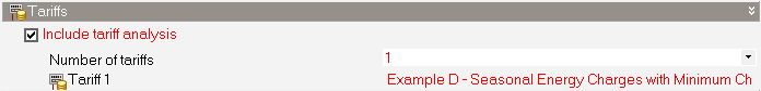
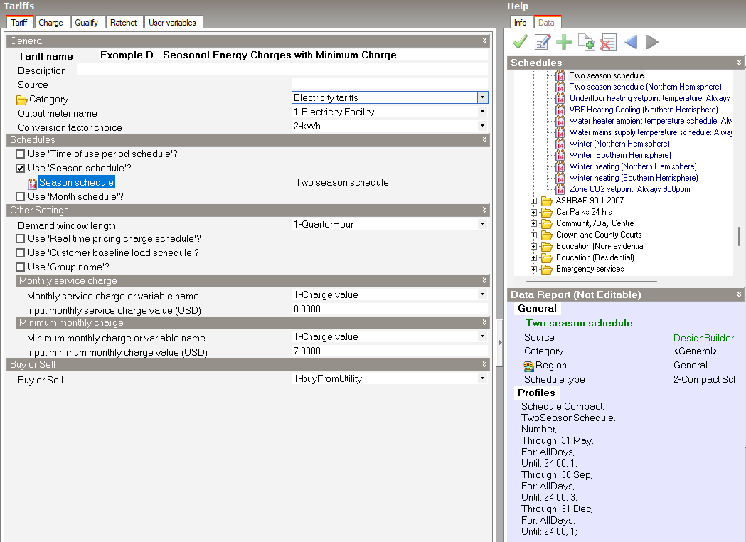
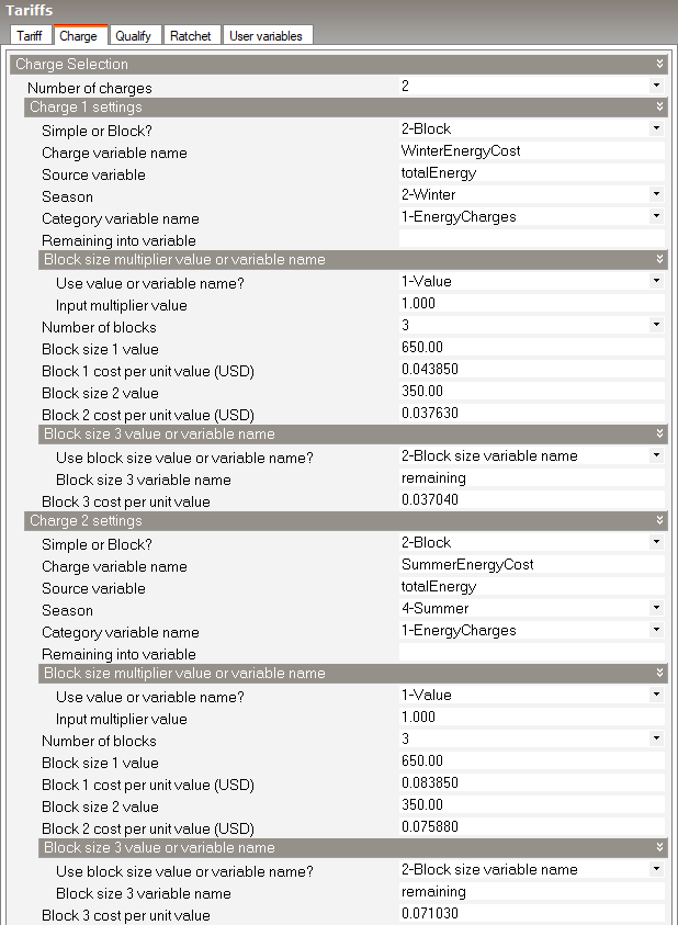
Utilities often have higher rates during peak seasons and minimum monthly charges to cover fixed costs. This example applies different block rates by season plus a minimum monthly fee. It is suitable for utilities with seasonal block structures (winter vs summer) and a guaranteed minimum bill.
Minimum charge: $7.00 per month
Winter – October through May, energy charges:
4.385 cents/kWh for first 650 kWh
3.763 cents/kWh for next 350 kWh
3.704 cents/kWh for over 1000 kWh
Summer – June through September, energy charges:
8.385 cents/kWh for first 650 kWh
7.588 cents/kWh for next 350 kWh
7.103 cents/kWh for over 1000 kWh
To create this tariff structure, follow the steps below.
1. Create a new Tariff component:
2. On the Tariff tab of the Tariff dialog:
Set the fixed monthly fee to $7.00 per month using the Input monthly service charge value setting.
Check the Use 'Season schedule' checkbox to reveal the Season schedule setting.
Create a new Seasonal schedule by copying the "Two season schedule (Northern Hemisphere)" library schedule. Call the new schedule "Two season schedule". The library schedule already contains the right settings, so for this example, no further changes are needed to the copy. But for other definitions of summer (e.g. in the Southern hemisphere) you should make the necessary edits to the copied schedule.
Select the newly created Seasonal schedule.
The Tariff tab should now look similar to the screenshot below.
3. On the Charge tab:
Set the Number of charges to 2, the first covering winter, the other for summer.
Under the Charge 1 settings header:
Set Simple or Block? to 2-Block.
Set Charge variable name to WinterEnergyCost
Set Source variable to totalEnergy
Set Season to 2-Winter.
Set the Number of blocks to 3
Set Block size 1 value to 650.
Set Block 1 cost per unit value to 0.04385 USD.
Set Block size 2 value to 350.
Set the Block 2 cost per unit value to 0.03763 USD.
Set the Block size 3 variable name to remaining.
Set the Block 3 cost per unit value to 0.03704 USD.
Under the Charge 2 settings header:
Set Simple or Block? to 2-Block.
Set Charge variable name to SummerEnergyCost
Set Source variable to totalEnergy
Set Season to 4-Summer.
Set the Number of blocks to 3
Set Block size 1 value to 650.
Set Block 1 cost per unit value to 0.08385 USD.
Set Block size 2 value to 350.
Set the Block 2 cost per unit value to 0.07588 USD.
Set the Block size 3 variable name to remaining.
Set the Block 3 cost per unit value to 0.07103 USD.
The screenshot below show how the charge tab should look when you have finished.
Report: Economics Results Summary Report
For: Entire Facility
Timestamp: 2025-09-11 11:38:13
Annual Cost
| Electricity | Natural Gas | Other | Total | |
| Cost [$] | 937.46 | 0.00 | 0.00 | 937.46 |
| Cost per Total Building Area [$/m2] | 5.13 | 0.00 | 0.00 | 5.13 |
| Cost per Net Conditioned Building Area [$/m2] | 5.13 | 0.00 | 0.00 | 5.13 |
Tariff Summary
| Selected | Qualified | Meter | Buy or Sell | Group | Annual Cost ($) | |
| ENERGYPLUS EXAMPLE D - SEASONAL ENERGY CHARGES WITH MINIMUM CHARGE | Yes | Yes | ELECTRICITY:FACILITY | Buy | (none) | 937.46 |
Report: Tariff Report
For: ENERGYPLUS EXAMPLE D - SEASONAL ENERGY CHARGES WITH MINIMUM CHARGE
Timestamp: 2025-09-11 11:38:13
General
| Parameter | |
| Meter | ELECTRICITY:FACILITY |
| Selected | Yes |
| Group | (none) |
| Qualified | Yes |
| Disqualifier | n/a |
| Computation | automatic |
| Units | kWh |
Categories
| Jan | Feb | Mar | Apr | May | Jun | Jul | Aug | Sep | Oct | Nov | Dec | Sum | Max | |
| EnergyCharges ($) | 51.33 | 45.87 | 49.55 | 57.72 | 67.33 | 118.08 | 141.34 | 132.85 | 117.29 | 58.05 | 48.44 | 49.61 | 937.46 | 141.34 |
| DemandCharges ($) | 0.00 | 0.00 | 0.00 | 0.00 | 0.00 | 0.00 | 0.00 | 0.00 | 0.00 | 0.00 | 0.00 | 0.00 | 0.00 | 0.00 |
| ServiceCharges ($) | 0.00 | 0.00 | 0.00 | 0.00 | 0.00 | 0.00 | 0.00 | 0.00 | 0.00 | 0.00 | 0.00 | 0.00 | 0.00 | 0.00 |
| Basis ($) | 51.33 | 45.87 | 49.55 | 57.72 | 67.33 | 118.08 | 141.34 | 132.85 | 117.29 | 58.05 | 48.44 | 49.61 | 937.46 | 141.34 |
| Adjustment ($) | 0.00 | 0.00 | 0.00 | 0.00 | 0.00 | 0.00 | 0.00 | 0.00 | 0.00 | 0.00 | 0.00 | 0.00 | 0.00 | 0.00 |
| Surcharge ($) | 0.00 | 0.00 | 0.00 | 0.00 | 0.00 | 0.00 | 0.00 | 0.00 | 0.00 | 0.00 | 0.00 | 0.00 | 0.00 | 0.00 |
| Subtotal ($) | 51.33 | 45.87 | 49.55 | 57.72 | 67.33 | 118.08 | 141.34 | 132.85 | 117.29 | 58.05 | 48.44 | 49.61 | 937.46 | 141.34 |
| Taxes ($) | 0.00 | 0.00 | 0.00 | 0.00 | 0.00 | 0.00 | 0.00 | 0.00 | 0.00 | 0.00 | 0.00 | 0.00 | 0.00 | 0.00 |
| Total ($) | 51.33 | 45.87 | 49.55 | 57.72 | 67.33 | 118.08 | 141.34 | 132.85 | 117.29 | 58.05 | 48.44 | 49.61 | 937.46 | 141.34 |
Charges
| Jan | Feb | Mar | Apr | May | Jun | Jul | Aug | Sep | Oct | Nov | Dec | Sum | Max | Category | |
| WINTERENERGYCOST ($) | 51.33 | 45.87 | 49.55 | 57.72 | 67.33 | 0.00 | 0.00 | 0.00 | 0.00 | 58.05 | 48.44 | 49.61 | 427.90 | 67.33 | EnergyCharges |
| SUMMERENERGYCOST ($) | 0.00 | 0.00 | 0.00 | 0.00 | 0.00 | 118.08 | 141.34 | 132.85 | 117.29 | 0.00 | 0.00 | 0.00 | 509.56 | 141.34 | EnergyCharges |
Corresponding Sources for Charges
| Jan | Feb | Mar | Apr | May | Jun | Jul | Aug | Sep | Oct | Nov | Dec | Sum | Max | |
| TotalEnergy | 1260.67 | 1113.39 | 1212.74 | 1433.24 | 1692.60 | 1521.19 | 1848.65 | 1729.11 | 1510.12 | 1442.16 | 1182.59 | 1214.35 | 17160.81 | 1848.65 |
Ratchets
| Jan | Feb | Mar | Apr | May | Jun | Jul | Aug | Sep | Oct | Nov | Dec | Sum | Max |
Qualifies
| Jan | Feb | Mar | Apr | May | Jun | Jul | Aug | Sep | Oct | Nov | Dec | Sum | Max |
Native Variables
| Jan | Feb | Mar | Apr | May | Jun | Jul | Aug | Sep | Oct | Nov | Dec | Sum | Max | |
| TotalEnergy | 1260.67 | 1113.39 | 1212.74 | 1433.24 | 1692.60 | 1521.19 | 1848.65 | 1729.11 | 1510.12 | 1442.16 | 1182.59 | 1214.35 | 17160.81 | 1848.65 |
| TotalDemand | 4.07 | 5.44 | 5.82 | 6.15 | 6.75 | 7.53 | 7.60 | 7.94 | 6.66 | 6.12 | 5.64 | 4.07 | 73.78 | 7.94 |
| PeakEnergy | 1260.67 | 1113.39 | 1212.74 | 1433.24 | 1692.60 | 1521.19 | 1848.65 | 1729.11 | 1510.12 | 1442.16 | 1182.59 | 1214.35 | 17160.81 | 1848.65 |
| PeakDemand | 4.07 | 5.44 | 5.82 | 6.15 | 6.75 | 7.53 | 7.60 | 7.94 | 6.66 | 6.12 | 5.64 | 4.07 | 73.78 | 7.94 |
| ShoulderEnergy | 0.00 | 0.00 | 0.00 | 0.00 | 0.00 | 0.00 | 0.00 | 0.00 | 0.00 | 0.00 | 0.00 | 0.00 | 0.00 | 0.00 |
| ShoulderDemand | 0.00 | 0.00 | 0.00 | 0.00 | 0.00 | 0.00 | 0.00 | 0.00 | 0.00 | 0.00 | 0.00 | 0.00 | 0.00 | 0.00 |
| OffPeakEnergy | 0.00 | 0.00 | 0.00 | 0.00 | 0.00 | 0.00 | 0.00 | 0.00 | 0.00 | 0.00 | 0.00 | 0.00 | 0.00 | 0.00 |
| OffPeakDemand | 0.00 | 0.00 | 0.00 | 0.00 | 0.00 | 0.00 | 0.00 | 0.00 | 0.00 | 0.00 | 0.00 | 0.00 | 0.00 | 0.00 |
| MidPeakEnergy | 0.00 | 0.00 | 0.00 | 0.00 | 0.00 | 0.00 | 0.00 | 0.00 | 0.00 | 0.00 | 0.00 | 0.00 | 0.00 | 0.00 |
| MidPeakDemand | 0.00 | 0.00 | 0.00 | 0.00 | 0.00 | 0.00 | 0.00 | 0.00 | 0.00 | 0.00 | 0.00 | 0.00 | 0.00 | 0.00 |
| PeakExceedsOffPeak | 4.07 | 5.44 | 5.82 | 6.15 | 6.75 | 7.53 | 7.60 | 7.94 | 6.66 | 6.12 | 5.64 | 4.07 | 73.78 | 7.94 |
| OffPeakExceedsPeak | 0.00 | 0.00 | 0.00 | 0.00 | 0.00 | 0.00 | 0.00 | 0.00 | 0.00 | 0.00 | 0.00 | 0.00 | 0.00 | 0.00 |
| PeakExceedsMidPeak | 4.07 | 5.44 | 5.82 | 6.15 | 6.75 | 7.53 | 7.60 | 7.94 | 6.66 | 6.12 | 5.64 | 4.07 | 73.78 | 7.94 |
| MidPeakExceedsPeak | 0.00 | 0.00 | 0.00 | 0.00 | 0.00 | 0.00 | 0.00 | 0.00 | 0.00 | 0.00 | 0.00 | 0.00 | 0.00 | 0.00 |
| PeakExceedsShoulder | 4.07 | 5.44 | 5.82 | 6.15 | 6.75 | 7.53 | 7.60 | 7.94 | 6.66 | 6.12 | 5.64 | 4.07 | 73.78 | 7.94 |
| ShoulderExceedsPeak | 0.00 | 0.00 | 0.00 | 0.00 | 0.00 | 0.00 | 0.00 | 0.00 | 0.00 | 0.00 | 0.00 | 0.00 | 0.00 | 0.00 |
| IsWinter | 1.00 | 1.00 | 1.00 | 1.00 | 1.00 | 0.00 | 0.00 | 0.00 | 0.00 | 1.00 | 1.00 | 1.00 | 8.00 | 1.00 |
| IsNotWinter | 0.00 | 0.00 | 0.00 | 0.00 | 0.00 | 1.00 | 1.00 | 1.00 | 1.00 | 0.00 | 0.00 | 0.00 | 4.00 | 1.00 |
| IsSpring | 0.00 | 0.00 | 0.00 | 0.00 | 0.00 | 0.00 | 0.00 | 0.00 | 0.00 | 0.00 | 0.00 | 0.00 | 0.00 | 0.00 |
| IsNotSpring | 1.00 | 1.00 | 1.00 | 1.00 | 1.00 | 1.00 | 1.00 | 1.00 | 1.00 | 1.00 | 1.00 | 1.00 | 12.00 | 1.00 |
| IsSummer | 0.00 | 0.00 | 0.00 | 0.00 | 0.00 | 1.00 | 1.00 | 1.00 | 1.00 | 0.00 | 0.00 | 0.00 | 4.00 | 1.00 |
| IsNotSummer | 1.00 | 1.00 | 1.00 | 1.00 | 1.00 | 0.00 | 0.00 | 0.00 | 0.00 | 1.00 | 1.00 | 1.00 | 8.00 | 1.00 |
| IsAutumn | 0.00 | 0.00 | 0.00 | 0.00 | 0.00 | 0.00 | 0.00 | 0.00 | 0.00 | 0.00 | 0.00 | 0.00 | 0.00 | 0.00 |
| IsNotAutumn | 1.00 | 1.00 | 1.00 | 1.00 | 1.00 | 1.00 | 1.00 | 1.00 | 1.00 | 1.00 | 1.00 | 1.00 | 12.00 | 1.00 |
| PeakAndShoulderEnergy | 1260.67 | 1113.39 | 1212.74 | 1433.24 | 1692.60 | 1521.19 | 1848.65 | 1729.11 | 1510.12 | 1442.16 | 1182.59 | 1214.35 | 17160.81 | 1848.65 |
| PeakAndShoulderDemand | 4.07 | 5.44 | 5.82 | 6.15 | 6.75 | 7.53 | 7.60 | 7.94 | 6.66 | 6.12 | 5.64 | 4.07 | 73.78 | 7.94 |
| PeakAndMidPeakEnergy | 1260.67 | 1113.39 | 1212.74 | 1433.24 | 1692.60 | 1521.19 | 1848.65 | 1729.11 | 1510.12 | 1442.16 | 1182.59 | 1214.35 | 17160.81 | 1848.65 |
| PeakAndMidPeakDemand | 4.07 | 5.44 | 5.82 | 6.15 | 6.75 | 7.53 | 7.60 | 7.94 | 6.66 | 6.12 | 5.64 | 4.07 | 73.78 | 7.94 |
| ShoulderAndOffPeakEnergy | 0.00 | 0.00 | 0.00 | 0.00 | 0.00 | 0.00 | 0.00 | 0.00 | 0.00 | 0.00 | 0.00 | 0.00 | 0.00 | 0.00 |
| ShoulderAndOffPeakDemand | 0.00 | 0.00 | 0.00 | 0.00 | 0.00 | 0.00 | 0.00 | 0.00 | 0.00 | 0.00 | 0.00 | 0.00 | 0.00 | 0.00 |
| PeakAndOffPeakEnergy | 1260.67 | 1113.39 | 1212.74 | 1433.24 | 1692.60 | 1521.19 | 1848.65 | 1729.11 | 1510.12 | 1442.16 | 1182.59 | 1214.35 | 17160.81 | 1848.65 |
| PeakAndOffPeakDemand | 4.07 | 5.44 | 5.82 | 6.15 | 6.75 | 7.53 | 7.60 | 7.94 | 6.66 | 6.12 | 5.64 | 4.07 | 73.78 | 7.94 |
| RealTimePriceCosts | 0.00 | 0.00 | 0.00 | 0.00 | 0.00 | 0.00 | 0.00 | 0.00 | 0.00 | 0.00 | 0.00 | 0.00 | 0.00 | 0.00 |
| AboveCustomerBaseCosts | 0.00 | 0.00 | 0.00 | 0.00 | 0.00 | 0.00 | 0.00 | 0.00 | 0.00 | 0.00 | 0.00 | 0.00 | 0.00 | 0.00 |
| BelowCustomerBaseCosts | 0.00 | 0.00 | 0.00 | 0.00 | 0.00 | 0.00 | 0.00 | 0.00 | 0.00 | 0.00 | 0.00 | 0.00 | 0.00 | 0.00 |
| AboveCustomerBaseEnergy | 0.00 | 0.00 | 0.00 | 0.00 | 0.00 | 0.00 | 0.00 | 0.00 | 0.00 | 0.00 | 0.00 | 0.00 | 0.00 | 0.00 |
| BelowCustomerBaseEnergy | 0.00 | 0.00 | 0.00 | 0.00 | 0.00 | 0.00 | 0.00 | 0.00 | 0.00 | 0.00 | 0.00 | 0.00 | 0.00 | 0.00 |
This example shows how to model a more sophisticated rate structure which encourages efficient energy use by linking energy pricing to monthly demand levels. Higher load factors (more consistent energy use) receive better rates. Energy blocks are multiplied by monthly peak demand to reflect load factor incentives. Such tariffs may be offered when customers with consistent energy use are more cost-effective to serve.
Customer charge: $14.00 per month
Energy charges:
8.756 cents/kWh for all consumption not greater than 200 hours times the demand
6.812 cents/kWh for all consumption in excess of 200 hours and not greater than 400 hours times the demand
5.029 cents/kWh for all consumption in excess of 400 hours times the demand.
This tariff uses a single Charge object. The monthly charge is defined on the Tariff tab. In this case the Block size multiplier is set to the totalDemand variable.
To create this tariff structure, follow the steps below.
1. Create a new Tariff component:
2. On the Tariff tab of the Tariff dialog:
Set the fixed monthly fee to $14.00 per month using the Input monthly service charge value setting.
The Tariff tab should now look similar to the screenshot below:
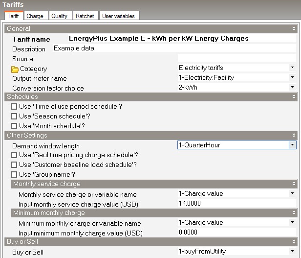
3. On the Charge tab:
Set the Number of charges to 1 to cover energy use.
Under the Charge 1 settings header:
Set Simple or Block? to 2-Block.
Set Charge variable name to BlockEnergyCharge
Set Source variable to totalEnergy
Under the Block size multiplier or variable name header, set Use value or variable name to totalDemand to indicate that block size values entered below are to be multiplied by the demand in kW.
Set the Number of blocks to 3
Set Block size 1 value to 200.
Set Block 1 cost per unit value to 0.08756 USD.
Set Block size 2 value to 200.
Set the Block 2 cost per unit value to 0.06812 USD.
Set the Block size 3 variable name to remaining.
Set the Block 3 cost per unit value to 0.05029 USD.
The Charge tab should now look similar to the screenshot below.
Report: Economics Results Summary Report
For: Entire Facility
Timestamp: 2025-09-11 11:30:42
Annual Cost
| Electricity | Natural Gas | Other | Total | |
| Cost [$] | 1623.87 | 0.00 | 0.00 | 1623.87 |
| Cost per Total Building Area [$/m2] | 8.88 | 0.00 | 0.00 | 8.88 |
| Cost per Net Conditioned Building Area [$/m2] | 8.88 | 0.00 | 0.00 | 8.88 |
Tariff Summary
| Selected | Qualified | Meter | Buy or Sell | Group | Annual Cost ($) | |
| ENERGYPLUS EXAMPLE E - KWH PER KW ENERGY CHARGES | Yes | Yes | ELECTRICITY:FACILITY | Buy | (none) | 1623.87 |
Report: Tariff Report
For: ENERGYPLUS EXAMPLE E - KWH PER KW ENERGY CHARGES
Timestamp: 2025-09-11 11:30:42
General
| Parameter | |
| Meter | ELECTRICITY:FACILITY |
| Selected | Yes |
| Group | (none) |
| Qualified | Yes |
| Disqualifier | n/a |
| Computation | automatic |
| Units | kWh |
Categories
| Jan | Feb | Mar | Apr | May | Jun | Jul | Aug | Sep | Oct | Nov | Dec | Sum | Max | |
| EnergyCharges ($) | 101.70 | 97.00 | 105.23 | 121.56 | 141.53 | 132.89 | 155.48 | 148.67 | 128.76 | 122.03 | 102.48 | 98.54 | 1455.87 | 155.48 |
| DemandCharges ($) | 0.00 | 0.00 | 0.00 | 0.00 | 0.00 | 0.00 | 0.00 | 0.00 | 0.00 | 0.00 | 0.00 | 0.00 | 0.00 | 0.00 |
| ServiceCharges ($) | 14.00 | 14.00 | 14.00 | 14.00 | 14.00 | 14.00 | 14.00 | 14.00 | 14.00 | 14.00 | 14.00 | 14.00 | 168.00 | 14.00 |
| Basis ($) | 115.70 | 111.00 | 119.23 | 135.56 | 155.53 | 146.89 | 169.48 | 162.67 | 142.76 | 136.03 | 116.48 | 112.54 | 1623.87 | 169.48 |
| Adjustment ($) | 0.00 | 0.00 | 0.00 | 0.00 | 0.00 | 0.00 | 0.00 | 0.00 | 0.00 | 0.00 | 0.00 | 0.00 | 0.00 | 0.00 |
| Surcharge ($) | 0.00 | 0.00 | 0.00 | 0.00 | 0.00 | 0.00 | 0.00 | 0.00 | 0.00 | 0.00 | 0.00 | 0.00 | 0.00 | 0.00 |
| Subtotal ($) | 115.70 | 111.00 | 119.23 | 135.56 | 155.53 | 146.89 | 169.48 | 162.67 | 142.76 | 136.03 | 116.48 | 112.54 | 1623.87 | 169.48 |
| Taxes ($) | 0.00 | 0.00 | 0.00 | 0.00 | 0.00 | 0.00 | 0.00 | 0.00 | 0.00 | 0.00 | 0.00 | 0.00 | 0.00 | 0.00 |
| Total ($) | 115.70 | 111.00 | 119.23 | 135.56 | 155.53 | 146.89 | 169.48 | 162.67 | 142.76 | 136.03 | 116.48 | 112.54 | 1623.87 | 169.48 |
Charges
| Jan | Feb | Mar | Apr | May | Jun | Jul | Aug | Sep | Oct | Nov | Dec | Sum | Max | Category | |
| BLOCKENERGYCHARGE ($) | 101.70 | 97.00 | 105.23 | 121.56 | 141.53 | 132.89 | 155.48 | 148.67 | 128.76 | 122.03 | 102.48 | 98.54 | 1455.87 | 155.48 | EnergyCharges |
Corresponding Sources for Charges
| Jan | Feb | Mar | Apr | May | Jun | Jul | Aug | Sep | Oct | Nov | Dec | Sum | Max | |
| TotalEnergy | 1260.67 | 1113.39 | 1212.74 | 1433.24 | 1692.60 | 1521.19 | 1848.65 | 1729.11 | 1510.12 | 1442.16 | 1182.59 | 1214.35 | 17160.81 | 1848.65 |
Ratchets
| Jan | Feb | Mar | Apr | May | Jun | Jul | Aug | Sep | Oct | Nov | Dec | Sum | Max |
Qualifies
| Jan | Feb | Mar | Apr | May | Jun | Jul | Aug | Sep | Oct | Nov | Dec | Sum | Max |
Native Variables
| Jan | Feb | Mar | Apr | May | Jun | Jul | Aug | Sep | Oct | Nov | Dec | Sum | Max | |
| TotalEnergy | 1260.67 | 1113.39 | 1212.74 | 1433.24 | 1692.60 | 1521.19 | 1848.65 | 1729.11 | 1510.12 | 1442.16 | 1182.59 | 1214.35 | 17160.81 | 1848.65 |
| TotalDemand | 4.07 | 5.44 | 5.82 | 6.15 | 6.75 | 7.53 | 7.60 | 7.94 | 6.66 | 6.12 | 5.64 | 4.07 | 73.78 | 7.94 |
| PeakEnergy | 1260.67 | 1113.39 | 1212.74 | 1433.24 | 1692.60 | 1521.19 | 1848.65 | 1729.11 | 1510.12 | 1442.16 | 1182.59 | 1214.35 | 17160.81 | 1848.65 |
| PeakDemand | 4.07 | 5.44 | 5.82 | 6.15 | 6.75 | 7.53 | 7.60 | 7.94 | 6.66 | 6.12 | 5.64 | 4.07 | 73.78 | 7.94 |
| ShoulderEnergy | 0.00 | 0.00 | 0.00 | 0.00 | 0.00 | 0.00 | 0.00 | 0.00 | 0.00 | 0.00 | 0.00 | 0.00 | 0.00 | 0.00 |
| ShoulderDemand | 0.00 | 0.00 | 0.00 | 0.00 | 0.00 | 0.00 | 0.00 | 0.00 | 0.00 | 0.00 | 0.00 | 0.00 | 0.00 | 0.00 |
| OffPeakEnergy | 0.00 | 0.00 | 0.00 | 0.00 | 0.00 | 0.00 | 0.00 | 0.00 | 0.00 | 0.00 | 0.00 | 0.00 | 0.00 | 0.00 |
| OffPeakDemand | 0.00 | 0.00 | 0.00 | 0.00 | 0.00 | 0.00 | 0.00 | 0.00 | 0.00 | 0.00 | 0.00 | 0.00 | 0.00 | 0.00 |
| MidPeakEnergy | 0.00 | 0.00 | 0.00 | 0.00 | 0.00 | 0.00 | 0.00 | 0.00 | 0.00 | 0.00 | 0.00 | 0.00 | 0.00 | 0.00 |
| MidPeakDemand | 0.00 | 0.00 | 0.00 | 0.00 | 0.00 | 0.00 | 0.00 | 0.00 | 0.00 | 0.00 | 0.00 | 0.00 | 0.00 | 0.00 |
| PeakExceedsOffPeak | 4.07 | 5.44 | 5.82 | 6.15 | 6.75 | 7.53 | 7.60 | 7.94 | 6.66 | 6.12 | 5.64 | 4.07 | 73.78 | 7.94 |
| OffPeakExceedsPeak | 0.00 | 0.00 | 0.00 | 0.00 | 0.00 | 0.00 | 0.00 | 0.00 | 0.00 | 0.00 | 0.00 | 0.00 | 0.00 | 0.00 |
| PeakExceedsMidPeak | 4.07 | 5.44 | 5.82 | 6.15 | 6.75 | 7.53 | 7.60 | 7.94 | 6.66 | 6.12 | 5.64 | 4.07 | 73.78 | 7.94 |
| MidPeakExceedsPeak | 0.00 | 0.00 | 0.00 | 0.00 | 0.00 | 0.00 | 0.00 | 0.00 | 0.00 | 0.00 | 0.00 | 0.00 | 0.00 | 0.00 |
| PeakExceedsShoulder | 4.07 | 5.44 | 5.82 | 6.15 | 6.75 | 7.53 | 7.60 | 7.94 | 6.66 | 6.12 | 5.64 | 4.07 | 73.78 | 7.94 |
| ShoulderExceedsPeak | 0.00 | 0.00 | 0.00 | 0.00 | 0.00 | 0.00 | 0.00 | 0.00 | 0.00 | 0.00 | 0.00 | 0.00 | 0.00 | 0.00 |
| IsWinter | 1.00 | 1.00 | 1.00 | 1.00 | 1.00 | 1.00 | 1.00 | 1.00 | 1.00 | 1.00 | 1.00 | 1.00 | 12.00 | 1.00 |
| IsNotWinter | 0.00 | 0.00 | 0.00 | 0.00 | 0.00 | 0.00 | 0.00 | 0.00 | 0.00 | 0.00 | 0.00 | 0.00 | 0.00 | 0.00 |
| IsSpring | 0.00 | 0.00 | 0.00 | 0.00 | 0.00 | 0.00 | 0.00 | 0.00 | 0.00 | 0.00 | 0.00 | 0.00 | 0.00 | 0.00 |
| IsNotSpring | 1.00 | 1.00 | 1.00 | 1.00 | 1.00 | 1.00 | 1.00 | 1.00 | 1.00 | 1.00 | 1.00 | 1.00 | 12.00 | 1.00 |
| IsSummer | 0.00 | 0.00 | 0.00 | 0.00 | 0.00 | 0.00 | 0.00 | 0.00 | 0.00 | 0.00 | 0.00 | 0.00 | 0.00 | 0.00 |
| IsNotSummer | 1.00 | 1.00 | 1.00 | 1.00 | 1.00 | 1.00 | 1.00 | 1.00 | 1.00 | 1.00 | 1.00 | 1.00 | 12.00 | 1.00 |
| IsAutumn | 0.00 | 0.00 | 0.00 | 0.00 | 0.00 | 0.00 | 0.00 | 0.00 | 0.00 | 0.00 | 0.00 | 0.00 | 0.00 | 0.00 |
| IsNotAutumn | 1.00 | 1.00 | 1.00 | 1.00 | 1.00 | 1.00 | 1.00 | 1.00 | 1.00 | 1.00 | 1.00 | 1.00 | 12.00 | 1.00 |
| PeakAndShoulderEnergy | 1260.67 | 1113.39 | 1212.74 | 1433.24 | 1692.60 | 1521.19 | 1848.65 | 1729.11 | 1510.12 | 1442.16 | 1182.59 | 1214.35 | 17160.81 | 1848.65 |
| PeakAndShoulderDemand | 4.07 | 5.44 | 5.82 | 6.15 | 6.75 | 7.53 | 7.60 | 7.94 | 6.66 | 6.12 | 5.64 | 4.07 | 73.78 | 7.94 |
| PeakAndMidPeakEnergy | 1260.67 | 1113.39 | 1212.74 | 1433.24 | 1692.60 | 1521.19 | 1848.65 | 1729.11 | 1510.12 | 1442.16 | 1182.59 | 1214.35 | 17160.81 | 1848.65 |
| PeakAndMidPeakDemand | 4.07 | 5.44 | 5.82 | 6.15 | 6.75 | 7.53 | 7.60 | 7.94 | 6.66 | 6.12 | 5.64 | 4.07 | 73.78 | 7.94 |
| ShoulderAndOffPeakEnergy | 0.00 | 0.00 | 0.00 | 0.00 | 0.00 | 0.00 | 0.00 | 0.00 | 0.00 | 0.00 | 0.00 | 0.00 | 0.00 | 0.00 |
| ShoulderAndOffPeakDemand | 0.00 | 0.00 | 0.00 | 0.00 | 0.00 | 0.00 | 0.00 | 0.00 | 0.00 | 0.00 | 0.00 | 0.00 | 0.00 | 0.00 |
| PeakAndOffPeakEnergy | 1260.67 | 1113.39 | 1212.74 | 1433.24 | 1692.60 | 1521.19 | 1848.65 | 1729.11 | 1510.12 | 1442.16 | 1182.59 | 1214.35 | 17160.81 | 1848.65 |
| PeakAndOffPeakDemand | 4.07 | 5.44 | 5.82 | 6.15 | 6.75 | 7.53 | 7.60 | 7.94 | 6.66 | 6.12 | 5.64 | 4.07 | 73.78 | 7.94 |
| RealTimePriceCosts | 0.00 | 0.00 | 0.00 | 0.00 | 0.00 | 0.00 | 0.00 | 0.00 | 0.00 | 0.00 | 0.00 | 0.00 | 0.00 | 0.00 |
| AboveCustomerBaseCosts | 0.00 | 0.00 | 0.00 | 0.00 | 0.00 | 0.00 | 0.00 | 0.00 | 0.00 | 0.00 | 0.00 | 0.00 | 0.00 | 0.00 |
| BelowCustomerBaseCosts | 0.00 | 0.00 | 0.00 | 0.00 | 0.00 | 0.00 | 0.00 | 0.00 | 0.00 | 0.00 | 0.00 | 0.00 | 0.00 | 0.00 |
| AboveCustomerBaseEnergy | 0.00 | 0.00 | 0.00 | 0.00 | 0.00 | 0.00 | 0.00 | 0.00 | 0.00 | 0.00 | 0.00 | 0.00 | 0.00 | 0.00 |
| BelowCustomerBaseEnergy | 0.00 | 0.00 | 0.00 | 0.00 | 0.00 | 0.00 | 0.00 | 0.00 | 0.00 | 0.00 | 0.00 | 0.00 | 0.00 | 0.00 |
Utilities face different costs throughout the day and year. Time-of-use rates pass these cost variations on to customers, encouraging usage during low-cost periods and discouraging use during high-cost periods. For example, tariffs sometimes have higher costs for energy consumed during the daytime than at night. In this example, four simple rates combine to create on-peak/off-peak and summer/winter distinctions. This approach is suitable for time-of-use tariffs where rates vary by both season and time of day.
Monthly charge: $37.75 per month
Winter – October through May
On Peak: 8.315 cents/kWh
Off-Peak: 2.420 cents/kWh
Summer – June through September
On Peak: 14.009 cents/kWh
Off-Peak: 6.312 cents/kWh
The on-peak period is defined as the hours starting at 10am and ending at 7pm, Monday through Friday for June through September and 3pm to 10pm Monday through Friday for October through May. All other hours are considered off-peak.
The tariff is only applicable for customers that use 50KW for at least one month of the year. This restriction is implemented by entering details on the Qualify tab.
This tariff uses four different Charge:Simple objects to capture the variation of energy cost with time.
To create this tariff structure, follow the steps below.
1. Create a new Tariff component:
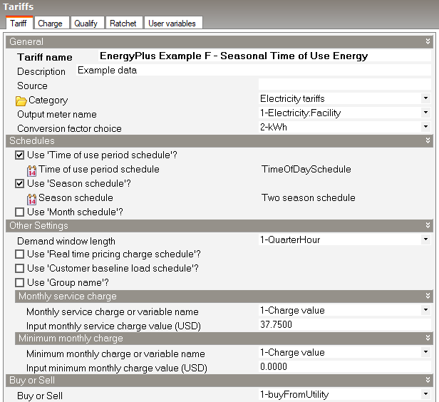
2. On the Tariff tab of the Tariff dialog:
Set the fixed monthly fee to $37.75 per month using the Input monthly service charge value setting.
Check the Use 'Time of use period schedule'? checkbox.
Use the Time of use period schedule, to define the on peak and off peak times. You can base your schedule on the library "Time of day schedule" by copying it, renaming the new schedule "TimeOfDaySchedule" and making any changes needed. As it happens the schedule shouldn't need any changes. It should look like the screenshot below.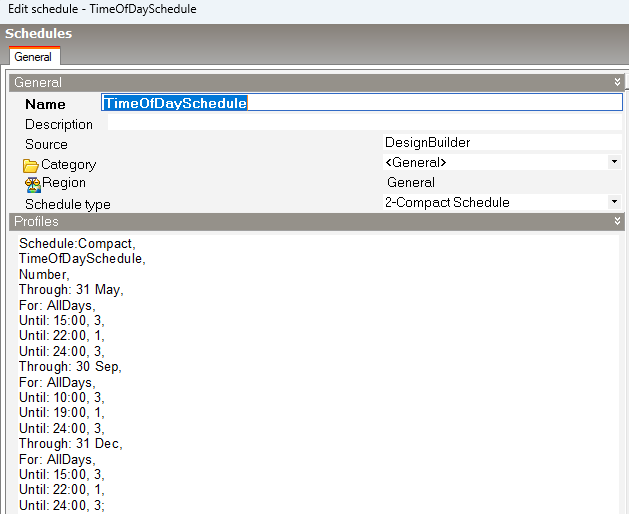
Check the Use 'Season schedule' checkbox to reveal the Season schedule setting.
Create a new Seasonal schedule by copying the "Two season schedule (Northern Hemisphere)" library schedule. Call the new schedule "Two season schedule". The library schedule already contains the right settings, so for this example, no further changes are needed to the copy. But for other definitions of summer (e.g. in the Southern hemisphere) you should make the necessary edits to the copied schedule.
Select the newly created Seasonal schedule.
The Tariff tab should now look similar to the screenshot below:
3. On the Charge tab:
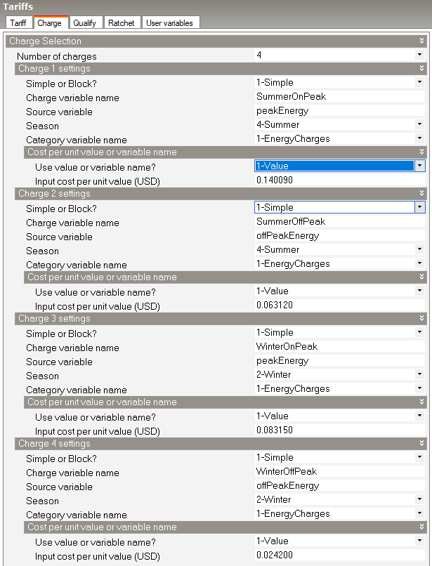
Set the Number of charges to 4 to cover the summer/winter on-peak/off-peak cases.
Under the Charge 1 settings header:
Set Simple or Block? to 1-Simple.
Set Charge variable name to SummerOnPeak
Set Source variable to peakEnergy
Set Season to 4-Summer
Set Category variable name to 1-EnergyCharges
Enter the Input cost per unit value as 0.14009
Under the Charge 2 settings header:
Set Simple or Block? to 1-Simple.
Set Charge variable name to SummerOffPeak
Set Source variable to offPeakEnergy
Set Season to 4-Summer
Set Category variable name to 1-EnergyCharges
Enter the Input cost per unit value as 0.06312
Under the Charge 3 settings header:
Set Simple or Block? to 1-Simple.
Set Charge variable name to WinterOnPeak
Set Source variable to peakEnergy
Set Season to 2-Winter
Set Category variable name to 1-EnergyCharges
Enter the Input cost per unit value as 0.08315
Under the Charge 4 settings header:
Set Simple or Block? to 1-Simple.
Set Charge variable name to WinterOffPeak
Set Source variable to offPeakEnergy
Set Season to 2-Winter
Set Category variable name to 1-EnergyCharges
Enter the Input cost per unit value as 0.02420
The Charge tab should now look similar to the screenshot below.
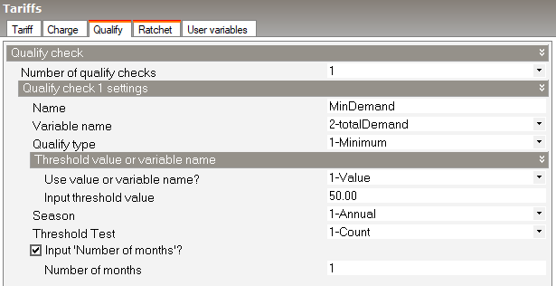
On the Qualify tab:
Set the Number of qualify checks to 1 to allow the minimum demand requirement.
Under the Qualify check 1 settings header:
Set the Name to MinDemand
Set the Variable name to 2-totalDemand
Set Qualify type to 1-Minimum
Enter the Input threshold value as 50
Set Season to 1-Annual
Set Threshold test to 1-Count
Check the Input 'Number of months'? checkbox
Set the Number of months to 1.
The Qualify tab should now look similar to the screenshot below.
Report: Economics Results Summary Report
For: Entire Facility
Timestamp: 2025-09-11 11:27:02
Annual Cost
| Electricity | Natural Gas | Other | Total | |
| Cost [$] | 0.00 | 0.00 | 0.00 | 0.00 |
| Cost per Total Building Area [$/m2] | 0.00 | 0.00 | 0.00 | 0.00 |
| Cost per Net Conditioned Building Area [$/m2] | 0.00 | 0.00 | 0.00 | 0.00 |
Tariff Summary
| Selected | Qualified | Meter | Buy or Sell | Group | Annual Cost ($) | |
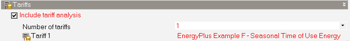
| ENERGYPLUS EXAMPLE F - SEASONAL TIME OF USE ENERGY | No | No | ELECTRICITY:FACILITY | Buy | (none) | 1707.55 |
Report: Tariff Report
For: ENERGYPLUS EXAMPLE F - SEASONAL TIME OF USE ENERGY
Timestamp: 2025-09-11 11:27:02
General
| Parameter | |
| Meter | ELECTRICITY:FACILITY |
| Selected | No |
| Group | (none) |
| Qualified | No |
| Disqualifier | MINDEMAND |
| Computation | automatic |
| Units | kWh |
Categories
| Jan | Feb | Mar | Apr | May | Jun | Jul | Aug | Sep | Oct | Nov | Dec | Sum | Max | |
| EnergyCharges ($) | 55.72 | 49.12 | 53.82 | 65.19 | 76.57 | 180.73 | 218.27 | 204.99 | 180.22 | 64.30 | 52.00 | 53.64 | 1254.55 | 218.27 |
| DemandCharges ($) | 0.00 | 0.00 | 0.00 | 0.00 | 0.00 | 0.00 | 0.00 | 0.00 | 0.00 | 0.00 | 0.00 | 0.00 | 0.00 | 0.00 |
| ServiceCharges ($) | 37.75 | 37.75 | 37.75 | 37.75 | 37.75 | 37.75 | 37.75 | 37.75 | 37.75 | 37.75 | 37.75 | 37.75 | 453.00 | 37.75 |
| Basis ($) | 93.47 | 86.87 | 91.57 | 102.94 | 114.32 | 218.48 | 256.02 | 242.74 | 217.97 | 102.05 | 89.75 | 91.39 | 1707.55 | 256.02 |
| Adjustment ($) | 0.00 | 0.00 | 0.00 | 0.00 | 0.00 | 0.00 | 0.00 | 0.00 | 0.00 | 0.00 | 0.00 | 0.00 | 0.00 | 0.00 |
| Surcharge ($) | 0.00 | 0.00 | 0.00 | 0.00 | 0.00 | 0.00 | 0.00 | 0.00 | 0.00 | 0.00 | 0.00 | 0.00 | 0.00 | 0.00 |
| Subtotal ($) | 93.47 | 86.87 | 91.57 | 102.94 | 114.32 | 218.48 | 256.02 | 242.74 | 217.97 | 102.05 | 89.75 | 91.39 | 1707.55 | 256.02 |
| Taxes ($) | 0.00 | 0.00 | 0.00 | 0.00 | 0.00 | 0.00 | 0.00 | 0.00 | 0.00 | 0.00 | 0.00 | 0.00 | 0.00 | 0.00 |
| Total ($) | 93.47 | 86.87 | 91.57 | 102.94 | 114.32 | 218.48 | 256.02 | 242.74 | 217.97 | 102.05 | 89.75 | 91.39 | 1707.55 | 256.02 |
Charges
| Jan | Feb | Mar | Apr | May | Jun | Jul | Aug | Sep | Oct | Nov | Dec | Sum | Max | Category | |
| SUMMERONPEAK ($) | 0.00 | 0.00 | 0.00 | 0.00 | 0.00 | 154.19 | 184.88 | 174.44 | 154.53 | 0.00 | 0.00 | 0.00 | 668.04 | 184.88 | EnergyCharges |
| SUMMEROFFPEAK ($) | 0.00 | 0.00 | 0.00 | 0.00 | 0.00 | 26.55 | 33.38 | 30.54 | 25.69 | 0.00 | 0.00 | 0.00 | 116.17 | 33.38 | EnergyCharges |
| WINTERONPEAK ($) | 35.55 | 31.27 | 34.52 | 43.02 | 50.22 | 0.00 | 0.00 | 0.00 | 0.00 | 41.47 | 32.98 | 34.21 | 303.24 | 50.22 | EnergyCharges |
| WINTEROFFPEAK ($) | 20.16 | 17.84 | 19.30 | 22.16 | 26.34 | 0.00 | 0.00 | 0.00 | 0.00 | 22.83 | 19.02 | 19.43 | 167.10 | 26.34 | EnergyCharges |
Corresponding Sources for Charges
| Jan | Feb | Mar | Apr | May | Jun | Jul | Aug | Sep | Oct | Nov | Dec | Sum | Max | |
| PeakEnergy | 427.60 | 376.11 | 415.12 | 517.41 | 604.00 | 1100.63 | 1319.75 | 1245.23 | 1103.07 | 498.69 | 396.58 | 411.45 | 8415.64 | 1319.75 |
| OffPeakEnergy | 833.07 | 737.28 | 797.62 | 915.83 | 1088.60 | 420.56 | 528.90 | 483.88 | 407.05 | 943.47 | 786.01 | 802.90 | 8745.18 | 1088.60 |
Ratchets
| Jan | Feb | Mar | Apr | May | Jun | Jul | Aug | Sep | Oct | Nov | Dec | Sum | Max |
Qualifies
| Jan | Feb | Mar | Apr | May | Jun | Jul | Aug | Sep | Oct | Nov | Dec | Sum | Max | |
| MINDEMAND | 0.00 | 0.00 | 0.00 | 0.00 | 0.00 | 0.00 | 0.00 | 0.00 | 0.00 | 0.00 | 0.00 | 0.00 | 0.00 | 0.00 |
Native Variables
| Jan | Feb | Mar | Apr | May | Jun | Jul | Aug | Sep | Oct | Nov | Dec | Sum | Max | |
| TotalEnergy | 1260.67 | 1113.39 | 1212.74 | 1433.24 | 1692.60 | 1521.19 | 1848.65 | 1729.11 | 1510.12 | 1442.16 | 1182.59 | 1214.35 | 17160.81 | 1848.65 |
| TotalDemand | 4.07 | 5.44 | 5.82 | 6.15 | 6.75 | 7.53 | 7.60 | 7.94 | 6.66 | 6.12 | 5.64 | 4.07 | 73.78 | 7.94 |
| PeakEnergy | 427.60 | 376.11 | 415.12 | 517.41 | 604.00 | 1100.63 | 1319.75 | 1245.23 | 1103.07 | 498.69 | 396.58 | 411.45 | 8415.64 | 1319.75 |
| PeakDemand | 4.05 | 5.17 | 5.79 | 6.15 | 6.75 | 7.53 | 7.60 | 7.94 | 6.66 | 6.11 | 5.10 | 4.05 | 72.90 | 7.94 |
| ShoulderEnergy | 0.00 | 0.00 | 0.00 | 0.00 | 0.00 | 0.00 | 0.00 | 0.00 | 0.00 | 0.00 | 0.00 | 0.00 | 0.00 | 0.00 |
| ShoulderDemand | 0.00 | 0.00 | 0.00 | 0.00 | 0.00 | 0.00 | 0.00 | 0.00 | 0.00 | 0.00 | 0.00 | 0.00 | 0.00 | 0.00 |
| OffPeakEnergy | 833.07 | 737.28 | 797.62 | 915.83 | 1088.60 | 420.56 | 528.90 | 483.88 | 407.05 | 943.47 | 786.01 | 802.90 | 8745.18 | 1088.60 |
| OffPeakDemand | 4.07 | 5.44 | 5.82 | 6.15 | 6.73 | 6.25 | 6.54 | 6.62 | 5.87 | 6.12 | 5.64 | 4.07 | 69.32 | 6.73 |
| MidPeakEnergy | 0.00 | 0.00 | 0.00 | 0.00 | 0.00 | 0.00 | 0.00 | 0.00 | 0.00 | 0.00 | 0.00 | 0.00 | 0.00 | 0.00 |
| MidPeakDemand | 0.00 | 0.00 | 0.00 | 0.00 | 0.00 | 0.00 | 0.00 | 0.00 | 0.00 | 0.00 | 0.00 | 0.00 | 0.00 | 0.00 |
| PeakExceedsOffPeak | 0.00 | 0.00 | 0.00 | 0.0047 | 0.0173 | 1.28 | 1.06 | 1.33 | 0.7863 | 0.00 | 0.00 | 0.00 | 4.47 | 1.33 |
| OffPeakExceedsPeak | 0.0214 | 0.2718 | 0.0247 | 0.00 | 0.00 | 0.00 | 0.00 | 0.00 | 0.00 | 0.0091 | 0.5367 | 0.0220 | 0.89 | 0.54 |
| PeakExceedsMidPeak | 4.05 | 5.17 | 5.79 | 6.15 | 6.75 | 7.53 | 7.60 | 7.94 | 6.66 | 6.11 | 5.10 | 4.05 | 72.90 | 7.94 |
| MidPeakExceedsPeak | 0.00 | 0.00 | 0.00 | 0.00 | 0.00 | 0.00 | 0.00 | 0.00 | 0.00 | 0.00 | 0.00 | 0.00 | 0.00 | 0.00 |
| PeakExceedsShoulder | 4.05 | 5.17 | 5.79 | 6.15 | 6.75 | 7.53 | 7.60 | 7.94 | 6.66 | 6.11 | 5.10 | 4.05 | 72.90 | 7.94 |
| ShoulderExceedsPeak | 0.00 | 0.00 | 0.00 | 0.00 | 0.00 | 0.00 | 0.00 | 0.00 | 0.00 | 0.00 | 0.00 | 0.00 | 0.00 | 0.00 |
| IsWinter | 1.00 | 1.00 | 1.00 | 1.00 | 1.00 | 0.00 | 0.00 | 0.00 | 0.00 | 1.00 | 1.00 | 1.00 | 8.00 | 1.00 |
| IsNotWinter | 0.00 | 0.00 | 0.00 | 0.00 | 0.00 | 1.00 | 1.00 | 1.00 | 1.00 | 0.00 | 0.00 | 0.00 | 4.00 | 1.00 |
| IsSpring | 0.00 | 0.00 | 0.00 | 0.00 | 0.00 | 0.00 | 0.00 | 0.00 | 0.00 | 0.00 | 0.00 | 0.00 | 0.00 | 0.00 |
| IsNotSpring | 1.00 | 1.00 | 1.00 | 1.00 | 1.00 | 1.00 | 1.00 | 1.00 | 1.00 | 1.00 | 1.00 | 1.00 | 12.00 | 1.00 |
| IsSummer | 0.00 | 0.00 | 0.00 | 0.00 | 0.00 | 1.00 | 1.00 | 1.00 | 1.00 | 0.00 | 0.00 | 0.00 | 4.00 | 1.00 |
| IsNotSummer | 1.00 | 1.00 | 1.00 | 1.00 | 1.00 | 0.00 | 0.00 | 0.00 | 0.00 | 1.00 | 1.00 | 1.00 | 8.00 | 1.00 |
| IsAutumn | 0.00 | 0.00 | 0.00 | 0.00 | 0.00 | 0.00 | 0.00 | 0.00 | 0.00 | 0.00 | 0.00 | 0.00 | 0.00 | 0.00 |
| IsNotAutumn | 1.00 | 1.00 | 1.00 | 1.00 | 1.00 | 1.00 | 1.00 | 1.00 | 1.00 | 1.00 | 1.00 | 1.00 | 12.00 | 1.00 |
| PeakAndShoulderEnergy | 427.60 | 376.11 | 415.12 | 517.41 | 604.00 | 1100.63 | 1319.75 | 1245.23 | 1103.07 | 498.69 | 396.58 | 411.45 | 8415.64 | 1319.75 |
| PeakAndShoulderDemand | 4.05 | 5.17 | 5.79 | 6.15 | 6.75 | 7.53 | 7.60 | 7.94 | 6.66 | 6.11 | 5.10 | 4.05 | 72.90 | 7.94 |
| PeakAndMidPeakEnergy | 427.60 | 376.11 | 415.12 | 517.41 | 604.00 | 1100.63 | 1319.75 | 1245.23 | 1103.07 | 498.69 | 396.58 | 411.45 | 8415.64 | 1319.75 |
| PeakAndMidPeakDemand | 4.05 | 5.17 | 5.79 | 6.15 | 6.75 | 7.53 | 7.60 | 7.94 | 6.66 | 6.11 | 5.10 | 4.05 | 72.90 | 7.94 |
| ShoulderAndOffPeakEnergy | 833.07 | 737.28 | 797.62 | 915.83 | 1088.60 | 420.56 | 528.90 | 483.88 | 407.05 | 943.47 | 786.01 | 802.90 | 8745.18 | 1088.60 |
| ShoulderAndOffPeakDemand | 4.07 | 5.44 | 5.82 | 6.15 | 6.73 | 6.25 | 6.54 | 6.62 | 5.87 | 6.12 | 5.64 | 4.07 | 69.32 | 6.73 |
| PeakAndOffPeakEnergy | 1260.67 | 1113.39 | 1212.74 | 1433.24 | 1692.60 | 1521.19 | 1848.65 | 1729.11 | 1510.12 | 1442.16 | 1182.59 | 1214.35 | 17160.81 | 1848.65 |
| PeakAndOffPeakDemand | 4.07 | 5.44 | 5.82 | 6.15 | 6.75 | 7.53 | 7.60 | 7.94 | 6.66 | 6.12 | 5.64 | 4.07 | 73.78 | 7.94 |
| RealTimePriceCosts | 0.00 | 0.00 | 0.00 | 0.00 | 0.00 | 0.00 | 0.00 | 0.00 | 0.00 | 0.00 | 0.00 | 0.00 | 0.00 | 0.00 |
| AboveCustomerBaseCosts | 0.00 | 0.00 | 0.00 | 0.00 | 0.00 | 0.00 | 0.00 | 0.00 | 0.00 | 0.00 | 0.00 | 0.00 | 0.00 | 0.00 |
| BelowCustomerBaseCosts | 0.00 | 0.00 | 0.00 | 0.00 | 0.00 | 0.00 | 0.00 | 0.00 | 0.00 | 0.00 | 0.00 | 0.00 | 0.00 | 0.00 |
| AboveCustomerBaseEnergy | 0.00 | 0.00 | 0.00 | 0.00 | 0.00 | 0.00 | 0.00 | 0.00 | 0.00 | 0.00 | 0.00 | 0.00 | 0.00 | 0.00 |
| BelowCustomerBaseEnergy | 0.00 | 0.00 | 0.00 | 0.00 | 0.00 | 0.00 | 0.00 | 0.00 | 0.00 | 0.00 | 0.00 | 0.00 | 0.00 | 0.00 |
Some utilities create complex rate structures that combine load factor incentives with traditional tiered pricing. This requires nested block calculations. Example G shows how to implement nested block structures by first allocating a demand-scaled block, then applying standard blocks to the resulting subsets. It is suitable for modelling complex tariffs combining scaled demand blocks and traditional kWh tiers for advanced load factor management.
Monthly charge: $35 per month
Energy charges:
For all consumption not greater than 200 hours times the demand use:
10.32 cents/kWh for the first 1000 kWh
7.43 cents/kWh for the next 4000 kWh
6.23 cents/kWh for the next 5000 kWh
4.27 cents/kWh for the remaining kWh less than 200 hours times the demand
For all consumption in excess of 200 hours and not greater than 400 hours times the demand, use:
6.82 cents/kWh
For all consumption in excess of 400 hours times the demand, use:
5.03 cents/kWh
To set up “block within a block”, Charge:Block settings are made to separate out the first 200 kWh/kW. The “EnergyFirst200kWhPerkW” charge performs this. It uses demand to multiply the first block size by 200 and the cost for the block is simply 1 since it passes through the energy to the variable “EnergyFirst200kWhPerkW”. The remaining energy goes into the restOfEnergy variable as specified in the Remaining into variable. After this has been evaluated we have two new variables that hold energy. Each of these variables are then separately used in Charge:Block objects to evaluate the different parts of the example tariff. By using the Remaining into variable along with the concept of variables, many very complex tariffs may be modelled.
To create this tariff structure, follow the steps below.
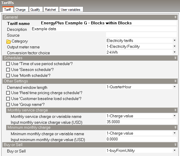
1. Create a new Tariff component:
2. On the Tariff tab of the Tariff dialog:
Set the fixed monthly fee to $35 per month using the Input monthly service charge value setting.
The Tariff tab should now look similar to the screenshot below:
3. On the Charge tab:
Set the Number of charges to 3.
Under the Charge 1 settings header:
Set Simple or Block? to 2-Block.
Set Charge variable name to EnergyFirst200kWhPerkW
Set Source variable to totalEnergy
Set Season to 1-Annual
Set Category variable name to 10-NotIncluded
Set Remaining into variable to restOfEnergy
Set Use value or variable name to 2-Variable name
Enter the Input multiplier variable name as totalDemand
Set Number of blocks to 1
Set Use block size value or variable name to 1-Block size value
Set Block size 1 value to 200
Set Block 1 cost per unit value to 1
Under the Charge 2 settings header:
Set Simple or Block? to 2-Block.
Set Charge variable name to CostOfFirst200kWhPerkW
Set Source variable to EnergyFirst200kWhPerkW
Set Season to 1-Annual
Set Category variable name to 1-EnergyCharges
Leave Remaining into variable blank
Set Use value or variable name to 1-Value
Set the Input multiplier value to 1
Set Number of blocks to 4
Set Use block size value or variable name to 1-Block size value
Set Block size 1 value to 1000
Set Block 1 cost per unit value to 0.103200
Set Block size 2 value to 4000
Set Block 2 cost per unit value to 0.074300
Set Block size 3 value to 5000
Set Block 3 cost per unit value to 0.062300
For Block 4, set Use block size value or variable name to 2-Block size variable name
Set Block size 4 variable name to remaining
Set Block 4 cost per unit value to 0.042700
Under the Charge 3 settings header:
Set Simple or Block? to 2-Block.
Set Charge variable name to CostOfRestOfEnergy
Set Source variable to restOfEnergy
Set Season to 1-Annual
Set Category variable name to 1-EnergyCharges
Leave Remaining into variable blank
Set Use value or variable name to 2-Variable name
Set the Input multiplier variable name to totalDemand
Set Number of blocks to 2
Set Use block size value or variable name to 1-Block size value
Set Block size 1 value to 200
Set Block 1 cost per unit value to 0.068200
For Block 2, set Use block size value or variable name to 2-Block size variable name
Set Block size 2 variable name to remaining
Set Block 2 cost per unit value to 0.050300
The Charge tab should now look similar to the screenshot below.
Report: Economics Results Summary Report
For: Entire Facility
Timestamp: 2025-09-11 11:18:57
Annual Cost
| Electricity | Natural Gas | Other | Total | |
| Cost [$] | 2016.42 | 0.00 | 0.00 | 2016.42 |
| Cost per Total Building Area [$/m2] | 11.03 | 0.00 | 0.00 | 11.03 |
| Cost per Net Conditioned Building Area [$/m2] | 11.03 | 0.00 | 0.00 | 11.03 |
Tariff Summary
| Selected | Qualified | Meter | Buy or Sell | Group | Annual Cost ($) | |
| ENERGYPLUS EXAMPLE G - BLOCKS WITHIN BLOCKS | Yes | Yes | ELECTRICITY:FACILITY | Buy | (none) | 2016.42 |
Report: Tariff Report
For: ENERGYPLUS EXAMPLE G - BLOCKS WITHIN BLOCKS
Timestamp: 2025-09-11 11:18:57
General
| Parameter | |
| Meter | ELECTRICITY:FACILITY |
| Selected | Yes |
| Group | (none) |
| Qualified | Yes |
| Disqualifier | n/a |
| Computation | automatic |
| Units | kWh |
Categories
| Jan | Feb | Mar | Apr | May | Jun | Jul | Aug | Sep | Oct | Nov | Dec | Sum | Max | |
| EnergyCharges ($) | 114.46 | 111.47 | 118.70 | 134.15 | 152.57 | 141.83 | 164.25 | 156.52 | 140.01 | 134.72 | 116.43 | 111.30 | 1596.42 | 164.25 |
| DemandCharges ($) | 0.00 | 0.00 | 0.00 | 0.00 | 0.00 | 0.00 | 0.00 | 0.00 | 0.00 | 0.00 | 0.00 | 0.00 | 0.00 | 0.00 |
| ServiceCharges ($) | 35.00 | 35.00 | 35.00 | 35.00 | 35.00 | 35.00 | 35.00 | 35.00 | 35.00 | 35.00 | 35.00 | 35.00 | 420.00 | 35.00 |
| Basis ($) | 149.46 | 146.47 | 153.70 | 169.15 | 187.57 | 176.83 | 199.25 | 191.52 | 175.01 | 169.72 | 151.43 | 146.30 | 2016.42 | 199.25 |
| Adjustment ($) | 0.00 | 0.00 | 0.00 | 0.00 | 0.00 | 0.00 | 0.00 | 0.00 | 0.00 | 0.00 | 0.00 | 0.00 | 0.00 | 0.00 |
| Surcharge ($) | 0.00 | 0.00 | 0.00 | 0.00 | 0.00 | 0.00 | 0.00 | 0.00 | 0.00 | 0.00 | 0.00 | 0.00 | 0.00 | 0.00 |
| Subtotal ($) | 149.46 | 146.47 | 153.70 | 169.15 | 187.57 | 176.83 | 199.25 | 191.52 | 175.01 | 169.72 | 151.43 | 146.30 | 2016.42 | 199.25 |
| Taxes ($) | 0.00 | 0.00 | 0.00 | 0.00 | 0.00 | 0.00 | 0.00 | 0.00 | 0.00 | 0.00 | 0.00 | 0.00 | 0.00 | 0.00 |
| Total ($) | 149.46 | 146.47 | 153.70 | 169.15 | 187.57 | 176.83 | 199.25 | 191.52 | 175.01 | 169.72 | 151.43 | 146.30 | 2016.42 | 199.25 |
Charges
| Jan | Feb | Mar | Apr | May | Jun | Jul | Aug | Sep | Oct | Nov | Dec | Sum | Max | Category | |
| ENERGYFIRST200KWHPERKW ($) | 813.74 | 1088.49 | 1163.30 | 1230.68 | 1349.17 | 1505.30 | 1520.17 | 1588.64 | 1331.93 | 1223.81 | 1127.85 | 813.75 | 14756.84 | 1588.64 | none |
| COSTOFFIRST200KWHPERKW ($) | 83.98 | 109.77 | 115.33 | 120.34 | 129.14 | 140.74 | 141.85 | 146.94 | 127.86 | 119.83 | 112.70 | 83.98 | 1432.47 | 146.94 | EnergyCharges |
| COSTOFRESTOFENERGY ($) | 30.48 | 1.70 | 3.37 | 13.82 | 23.42 | 1.08 | 22.40 | 9.58 | 12.15 | 14.89 | 3.73 | 27.32 | 163.95 | 30.48 | EnergyCharges |
Corresponding Sources for Charges
| Jan | Feb | Mar | Apr | May | Jun | Jul | Aug | Sep | Oct | Nov | Dec | Sum | Max | |
| TotalEnergy | 1260.67 | 1113.39 | 1212.74 | 1433.24 | 1692.60 | 1521.19 | 1848.65 | 1729.11 | 1510.12 | 1442.16 | 1182.59 | 1214.35 | 17160.81 | 1848.65 |
| ENERGYFIRST200KWHPERKW | 813.74 | 1088.49 | 1163.30 | 1230.68 | 1349.17 | 1505.30 | 1520.17 | 1588.64 | 1331.93 | 1223.81 | 1127.85 | 813.75 | 14756.84 | 1588.64 |
| RESTOFENERGY | 446.93 | 24.90 | 49.44 | 202.57 | 343.43 | 15.90 | 328.48 | 140.47 | 178.18 | 218.35 | 54.73 | 400.60 | 2403.98 | 446.93 |
Ratchets
| Jan | Feb | Mar | Apr | May | Jun | Jul | Aug | Sep | Oct | Nov | Dec | Sum | Max |
Qualifies
| Jan | Feb | Mar | Apr | May | Jun | Jul | Aug | Sep | Oct | Nov | Dec | Sum | Max |
Native Variables
| Jan | Feb | Mar | Apr | May | Jun | Jul | Aug | Sep | Oct | Nov | Dec | Sum | Max | |
| TotalEnergy | 1260.67 | 1113.39 | 1212.74 | 1433.24 | 1692.60 | 1521.19 | 1848.65 | 1729.11 | 1510.12 | 1442.16 | 1182.59 | 1214.35 | 17160.81 | 1848.65 |
| TotalDemand | 4.07 | 5.44 | 5.82 | 6.15 | 6.75 | 7.53 | 7.60 | 7.94 | 6.66 | 6.12 | 5.64 | 4.07 | 73.78 | 7.94 |
| PeakEnergy | 1260.67 | 1113.39 | 1212.74 | 1433.24 | 1692.60 | 1521.19 | 1848.65 | 1729.11 | 1510.12 | 1442.16 | 1182.59 | 1214.35 | 17160.81 | 1848.65 |
| PeakDemand | 4.07 | 5.44 | 5.82 | 6.15 | 6.75 | 7.53 | 7.60 | 7.94 | 6.66 | 6.12 | 5.64 | 4.07 | 73.78 | 7.94 |
| ShoulderEnergy | 0.00 | 0.00 | 0.00 | 0.00 | 0.00 | 0.00 | 0.00 | 0.00 | 0.00 | 0.00 | 0.00 | 0.00 | 0.00 | 0.00 |
| ShoulderDemand | 0.00 | 0.00 | 0.00 | 0.00 | 0.00 | 0.00 | 0.00 | 0.00 | 0.00 | 0.00 | 0.00 | 0.00 | 0.00 | 0.00 |
| OffPeakEnergy | 0.00 | 0.00 | 0.00 | 0.00 | 0.00 | 0.00 | 0.00 | 0.00 | 0.00 | 0.00 | 0.00 | 0.00 | 0.00 | 0.00 |
| OffPeakDemand | 0.00 | 0.00 | 0.00 | 0.00 | 0.00 | 0.00 | 0.00 | 0.00 | 0.00 | 0.00 | 0.00 | 0.00 | 0.00 | 0.00 |
| MidPeakEnergy | 0.00 | 0.00 | 0.00 | 0.00 | 0.00 | 0.00 | 0.00 | 0.00 | 0.00 | 0.00 | 0.00 | 0.00 | 0.00 | 0.00 |
| MidPeakDemand | 0.00 | 0.00 | 0.00 | 0.00 | 0.00 | 0.00 | 0.00 | 0.00 | 0.00 | 0.00 | 0.00 | 0.00 | 0.00 | 0.00 |
| PeakExceedsOffPeak | 4.07 | 5.44 | 5.82 | 6.15 | 6.75 | 7.53 | 7.60 | 7.94 | 6.66 | 6.12 | 5.64 | 4.07 | 73.78 | 7.94 |
| OffPeakExceedsPeak | 0.00 | 0.00 | 0.00 | 0.00 | 0.00 | 0.00 | 0.00 | 0.00 | 0.00 | 0.00 | 0.00 | 0.00 | 0.00 | 0.00 |
| PeakExceedsMidPeak | 4.07 | 5.44 | 5.82 | 6.15 | 6.75 | 7.53 | 7.60 | 7.94 | 6.66 | 6.12 | 5.64 | 4.07 | 73.78 | 7.94 |
| MidPeakExceedsPeak | 0.00 | 0.00 | 0.00 | 0.00 | 0.00 | 0.00 | 0.00 | 0.00 | 0.00 | 0.00 | 0.00 | 0.00 | 0.00 | 0.00 |
| PeakExceedsShoulder | 4.07 | 5.44 | 5.82 | 6.15 | 6.75 | 7.53 | 7.60 | 7.94 | 6.66 | 6.12 | 5.64 | 4.07 | 73.78 | 7.94 |
| ShoulderExceedsPeak | 0.00 | 0.00 | 0.00 | 0.00 | 0.00 | 0.00 | 0.00 | 0.00 | 0.00 | 0.00 | 0.00 | 0.00 | 0.00 | 0.00 |
| IsWinter | 1.00 | 1.00 | 1.00 | 1.00 | 1.00 | 1.00 | 1.00 | 1.00 | 1.00 | 1.00 | 1.00 | 1.00 | 12.00 | 1.00 |
| IsNotWinter | 0.00 | 0.00 | 0.00 | 0.00 | 0.00 | 0.00 | 0.00 | 0.00 | 0.00 | 0.00 | 0.00 | 0.00 | 0.00 | 0.00 |
| IsSpring | 0.00 | 0.00 | 0.00 | 0.00 | 0.00 | 0.00 | 0.00 | 0.00 | 0.00 | 0.00 | 0.00 | 0.00 | 0.00 | 0.00 |
| IsNotSpring | 1.00 | 1.00 | 1.00 | 1.00 | 1.00 | 1.00 | 1.00 | 1.00 | 1.00 | 1.00 | 1.00 | 1.00 | 12.00 | 1.00 |
| IsSummer | 0.00 | 0.00 | 0.00 | 0.00 | 0.00 | 0.00 | 0.00 | 0.00 | 0.00 | 0.00 | 0.00 | 0.00 | 0.00 | 0.00 |
| IsNotSummer | 1.00 | 1.00 | 1.00 | 1.00 | 1.00 | 1.00 | 1.00 | 1.00 | 1.00 | 1.00 | 1.00 | 1.00 | 12.00 | 1.00 |
| IsAutumn | 0.00 | 0.00 | 0.00 | 0.00 | 0.00 | 0.00 | 0.00 | 0.00 | 0.00 | 0.00 | 0.00 | 0.00 | 0.00 | 0.00 |
| IsNotAutumn | 1.00 | 1.00 | 1.00 | 1.00 | 1.00 | 1.00 | 1.00 | 1.00 | 1.00 | 1.00 | 1.00 | 1.00 | 12.00 | 1.00 |
| PeakAndShoulderEnergy | 1260.67 | 1113.39 | 1212.74 | 1433.24 | 1692.60 | 1521.19 | 1848.65 | 1729.11 | 1510.12 | 1442.16 | 1182.59 | 1214.35 | 17160.81 | 1848.65 |
| PeakAndShoulderDemand | 4.07 | 5.44 | 5.82 | 6.15 | 6.75 | 7.53 | 7.60 | 7.94 | 6.66 | 6.12 | 5.64 | 4.07 | 73.78 | 7.94 |
| PeakAndMidPeakEnergy | 1260.67 | 1113.39 | 1212.74 | 1433.24 | 1692.60 | 1521.19 | 1848.65 | 1729.11 | 1510.12 | 1442.16 | 1182.59 | 1214.35 | 17160.81 | 1848.65 |
| PeakAndMidPeakDemand | 4.07 | 5.44 | 5.82 | 6.15 | 6.75 | 7.53 | 7.60 | 7.94 | 6.66 | 6.12 | 5.64 | 4.07 | 73.78 | 7.94 |
| ShoulderAndOffPeakEnergy | 0.00 | 0.00 | 0.00 | 0.00 | 0.00 | 0.00 | 0.00 | 0.00 | 0.00 | 0.00 | 0.00 | 0.00 | 0.00 | 0.00 |
| ShoulderAndOffPeakDemand | 0.00 | 0.00 | 0.00 | 0.00 | 0.00 | 0.00 | 0.00 | 0.00 | 0.00 | 0.00 | 0.00 | 0.00 | 0.00 | 0.00 |
| PeakAndOffPeakEnergy | 1260.67 | 1113.39 | 1212.74 | 1433.24 | 1692.60 | 1521.19 | 1848.65 | 1729.11 | 1510.12 | 1442.16 | 1182.59 | 1214.35 | 17160.81 | 1848.65 |
| PeakAndOffPeakDemand | 4.07 | 5.44 | 5.82 | 6.15 | 6.75 | 7.53 | 7.60 | 7.94 | 6.66 | 6.12 | 5.64 | 4.07 | 73.78 | 7.94 |
| RealTimePriceCosts | 0.00 | 0.00 | 0.00 | 0.00 | 0.00 | 0.00 | 0.00 | 0.00 | 0.00 | 0.00 | 0.00 | 0.00 | 0.00 | 0.00 |
| AboveCustomerBaseCosts | 0.00 | 0.00 | 0.00 | 0.00 | 0.00 | 0.00 | 0.00 | 0.00 | 0.00 | 0.00 | 0.00 | 0.00 | 0.00 | 0.00 |
| BelowCustomerBaseCosts | 0.00 | 0.00 | 0.00 | 0.00 | 0.00 | 0.00 | 0.00 | 0.00 | 0.00 | 0.00 | 0.00 | 0.00 | 0.00 | 0.00 |
| AboveCustomerBaseEnergy | 0.00 | 0.00 | 0.00 | 0.00 | 0.00 | 0.00 | 0.00 | 0.00 | 0.00 | 0.00 | 0.00 | 0.00 | 0.00 | 0.00 |
| BelowCustomerBaseEnergy | 0.00 | 0.00 | 0.00 | 0.00 | 0.00 | 0.00 | 0.00 | 0.00 | 0.00 | 0.00 | 0.00 | 0.00 | 0.00 | 0.00 |
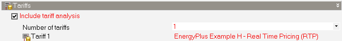
Some utilities offer hourly pricing that varies based on real-time market conditions which are typically announced day-ahead. Hourly energy prices are imported from a schedule, with no predefined charges. This example shows how to model real-time pricing tariffs where the utility provides hourly prices in advance.
To model this type of utility rate a schedule is used that contains the prices on an hourly basis. The Real time pricing charge schedule contains the prices and the Customer baseline load schedule setting is used to set the schedule for the customer baseline load. Not all utilities use a customer baseline load in which case this schedule does not need to be entered. The Period, Season and Month Schedules are not needed for these tariffs unless Charges are used.
The example real time pricing schedule results in the same energy cost as Example F – Seasonal Time of Use Energy. Note that this is only an example and usually for real time pricing the schedule values would vary throughout the year.
To create this tariff structure, follow the steps below.
1. Create a new Tariff component:
2. On the Tariff tab of the Tariff dialog:
Set the fixed monthly fee to $37.75 per month using the Input monthly service charge value setting.
Check the Use 'Real time pricing charge schedule'? checkbox.
Click on the Real time pricing charge schedule control and make a copy of the library schedule: "Real time pricing schedule". Name the copy of the schedule "RealTimePricing" and select it. The copied library schedule should already contain the right settings for this example, so for our purposes, no further changes are needed to the copy. The schedule should look like the screenshot below. Of course, for your project work, you would make the necessary edits to the copied schedule. 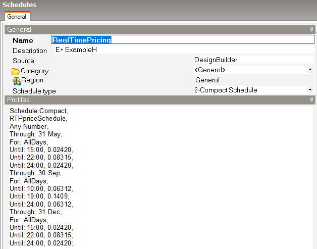
Select the newly created Real time schedule.
The Tariff tab should now look similar to the screenshot below:
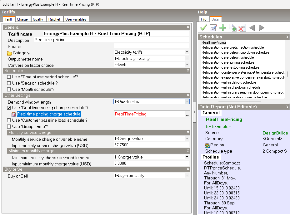
3. On the Charge tab of the Tariff dialog, there should be no charges, i.e. Number of charges should be set to 0. See below.
Report: Economics Results Summary Report
For: Entire Facility
Timestamp: 2025-09-11 11:24:51
Annual Cost
| Electricity | Natural Gas | Other | Total | |
| Cost [$] | 2016.42 | 0.00 | 0.00 | 2016.42 |
| Cost per Total Building Area [$/m2] | 11.03 | 0.00 | 0.00 | 11.03 |
| Cost per Net Conditioned Building Area [$/m2] | 11.03 | 0.00 | 0.00 | 11.03 |
Tariff Summary
| Selected | Qualified | Meter | Buy or Sell | Group | Annual Cost ($) | |
| ENERGYPLUS EXAMPLE G - BLOCKS WITHIN BLOCKS | Yes | Yes | ELECTRICITY:FACILITY | Buy | (none) | 2016.42 |
Report: Tariff Report
For: ENERGYPLUS EXAMPLE H - REAL TIME PRICING (RTP)
Timestamp: 2025-09-11 11:13:24
General
| Parameter | |
| Meter | ELECTRICITY:FACILITY |
| Selected | Yes |
| Group | (none) |
| Qualified | Yes |
| Disqualifier | n/a |
| Computation | automatic |
| Units | kWh |
Categories
| Jan | Feb | Mar | Apr | May | Jun | Jul | Aug | Sep | Oct | Nov | Dec | Sum | Max | |
| EnergyCharges ($) | 55.72 | 49.12 | 53.82 | 65.19 | 76.57 | 181.62 | 219.34 | 205.99 | 181.12 | 64.30 | 52.00 | 53.64 | 1258.41 | 219.34 |
| DemandCharges ($) | 0.00 | 0.00 | 0.00 | 0.00 | 0.00 | 0.00 | 0.00 | 0.00 | 0.00 | 0.00 | 0.00 | 0.00 | 0.00 | 0.00 |
| ServiceCharges ($) | 37.75 | 37.75 | 37.75 | 37.75 | 37.75 | 37.75 | 37.75 | 37.75 | 37.75 | 37.75 | 37.75 | 37.75 | 453.00 | 37.75 |
| Basis ($) | 93.47 | 86.87 | 91.57 | 102.94 | 114.32 | 219.37 | 257.09 | 243.74 | 218.87 | 102.05 | 89.75 | 91.39 | 1711.41 | 257.09 |
| Adjustment ($) | 0.00 | 0.00 | 0.00 | 0.00 | 0.00 | 0.00 | 0.00 | 0.00 | 0.00 | 0.00 | 0.00 | 0.00 | 0.00 | 0.00 |
| Surcharge ($) | 0.00 | 0.00 | 0.00 | 0.00 | 0.00 | 0.00 | 0.00 | 0.00 | 0.00 | 0.00 | 0.00 | 0.00 | 0.00 | 0.00 |
| Subtotal ($) | 93.47 | 86.87 | 91.57 | 102.94 | 114.32 | 219.37 | 257.09 | 243.74 | 218.87 | 102.05 | 89.75 | 91.39 | 1711.41 | 257.09 |
| Taxes ($) | 0.00 | 0.00 | 0.00 | 0.00 | 0.00 | 0.00 | 0.00 | 0.00 | 0.00 | 0.00 | 0.00 | 0.00 | 0.00 | 0.00 |
| Total ($) | 93.47 | 86.87 | 91.57 | 102.94 | 114.32 | 219.37 | 257.09 | 243.74 | 218.87 | 102.05 | 89.75 | 91.39 | 1711.41 | 257.09 |
Charges
| Jan | Feb | Mar | Apr | May | Jun | Jul | Aug | Sep | Oct | Nov | Dec | Sum | Max | Category |
Corresponding Sources for Charges
| Jan | Feb | Mar | Apr | May | Jun | Jul | Aug | Sep | Oct | Nov | Dec | Sum | Max |
Ratchets
| Jan | Feb | Mar | Apr | May | Jun | Jul | Aug | Sep | Oct | Nov | Dec | Sum | Max |
Qualifies
| Jan | Feb | Mar | Apr | May | Jun | Jul | Aug | Sep | Oct | Nov | Dec | Sum | Max |
Native Variables
| Jan | Feb | Mar | Apr | May | Jun | Jul | Aug | Sep | Oct | Nov | Dec | Sum | Max | |
| TotalEnergy | 1260.67 | 1113.39 | 1212.74 | 1433.24 | 1692.60 | 1521.19 | 1848.65 | 1729.11 | 1510.12 | 1442.16 | 1182.59 | 1214.35 | 17160.81 | 1848.65 |
| TotalDemand | 4.07 | 5.44 | 5.82 | 6.15 | 6.75 | 7.53 | 7.60 | 7.94 | 6.66 | 6.12 | 5.64 | 4.07 | 73.78 | 7.94 |
| PeakEnergy | 1260.67 | 1113.39 | 1212.74 | 1433.24 | 1692.60 | 1521.19 | 1848.65 | 1729.11 | 1510.12 | 1442.16 | 1182.59 | 1214.35 | 17160.81 | 1848.65 |
| PeakDemand | 4.07 | 5.44 | 5.82 | 6.15 | 6.75 | 7.53 | 7.60 | 7.94 | 6.66 | 6.12 | 5.64 | 4.07 | 73.78 | 7.94 |
| ShoulderEnergy | 0.00 | 0.00 | 0.00 | 0.00 | 0.00 | 0.00 | 0.00 | 0.00 | 0.00 | 0.00 | 0.00 | 0.00 | 0.00 | 0.00 |
| ShoulderDemand | 0.00 | 0.00 | 0.00 | 0.00 | 0.00 | 0.00 | 0.00 | 0.00 | 0.00 | 0.00 | 0.00 | 0.00 | 0.00 | 0.00 |
| OffPeakEnergy | 0.00 | 0.00 | 0.00 | 0.00 | 0.00 | 0.00 | 0.00 | 0.00 | 0.00 | 0.00 | 0.00 | 0.00 | 0.00 | 0.00 |
| OffPeakDemand | 0.00 | 0.00 | 0.00 | 0.00 | 0.00 | 0.00 | 0.00 | 0.00 | 0.00 | 0.00 | 0.00 | 0.00 | 0.00 | 0.00 |
| MidPeakEnergy | 0.00 | 0.00 | 0.00 | 0.00 | 0.00 | 0.00 | 0.00 | 0.00 | 0.00 | 0.00 | 0.00 | 0.00 | 0.00 | 0.00 |
| MidPeakDemand | 0.00 | 0.00 | 0.00 | 0.00 | 0.00 | 0.00 | 0.00 | 0.00 | 0.00 | 0.00 | 0.00 | 0.00 | 0.00 | 0.00 |
| PeakExceedsOffPeak | 4.07 | 5.44 | 5.82 | 6.15 | 6.75 | 7.53 | 7.60 | 7.94 | 6.66 | 6.12 | 5.64 | 4.07 | 73.78 | 7.94 |
| OffPeakExceedsPeak | 0.00 | 0.00 | 0.00 | 0.00 | 0.00 | 0.00 | 0.00 | 0.00 | 0.00 | 0.00 | 0.00 | 0.00 | 0.00 | 0.00 |
| PeakExceedsMidPeak | 4.07 | 5.44 | 5.82 | 6.15 | 6.75 | 7.53 | 7.60 | 7.94 | 6.66 | 6.12 | 5.64 | 4.07 | 73.78 | 7.94 |
| MidPeakExceedsPeak | 0.00 | 0.00 | 0.00 | 0.00 | 0.00 | 0.00 | 0.00 | 0.00 | 0.00 | 0.00 | 0.00 | 0.00 | 0.00 | 0.00 |
| PeakExceedsShoulder | 4.07 | 5.44 | 5.82 | 6.15 | 6.75 | 7.53 | 7.60 | 7.94 | 6.66 | 6.12 | 5.64 | 4.07 | 73.78 | 7.94 |
| ShoulderExceedsPeak | 0.00 | 0.00 | 0.00 | 0.00 | 0.00 | 0.00 | 0.00 | 0.00 | 0.00 | 0.00 | 0.00 | 0.00 | 0.00 | 0.00 |
| IsWinter | 1.00 | 1.00 | 1.00 | 1.00 | 1.00 | 1.00 | 1.00 | 1.00 | 1.00 | 1.00 | 1.00 | 1.00 | 12.00 | 1.00 |
| IsNotWinter | 0.00 | 0.00 | 0.00 | 0.00 | 0.00 | 0.00 | 0.00 | 0.00 | 0.00 | 0.00 | 0.00 | 0.00 | 0.00 | 0.00 |
| IsSpring | 0.00 | 0.00 | 0.00 | 0.00 | 0.00 | 0.00 | 0.00 | 0.00 | 0.00 | 0.00 | 0.00 | 0.00 | 0.00 | 0.00 |
| IsNotSpring | 1.00 | 1.00 | 1.00 | 1.00 | 1.00 | 1.00 | 1.00 | 1.00 | 1.00 | 1.00 | 1.00 | 1.00 | 12.00 | 1.00 |
| IsSummer | 0.00 | 0.00 | 0.00 | 0.00 | 0.00 | 0.00 | 0.00 | 0.00 | 0.00 | 0.00 | 0.00 | 0.00 | 0.00 | 0.00 |
| IsNotSummer | 1.00 | 1.00 | 1.00 | 1.00 | 1.00 | 1.00 | 1.00 | 1.00 | 1.00 | 1.00 | 1.00 | 1.00 | 12.00 | 1.00 |
| IsAutumn | 0.00 | 0.00 | 0.00 | 0.00 | 0.00 | 0.00 | 0.00 | 0.00 | 0.00 | 0.00 | 0.00 | 0.00 | 0.00 | 0.00 |
| IsNotAutumn | 1.00 | 1.00 | 1.00 | 1.00 | 1.00 | 1.00 | 1.00 | 1.00 | 1.00 | 1.00 | 1.00 | 1.00 | 12.00 | 1.00 |
| PeakAndShoulderEnergy | 1260.67 | 1113.39 | 1212.74 | 1433.24 | 1692.60 | 1521.19 | 1848.65 | 1729.11 | 1510.12 | 1442.16 | 1182.59 | 1214.35 | 17160.81 | 1848.65 |
| PeakAndShoulderDemand | 4.07 | 5.44 | 5.82 | 6.15 | 6.75 | 7.53 | 7.60 | 7.94 | 6.66 | 6.12 | 5.64 | 4.07 | 73.78 | 7.94 |
| PeakAndMidPeakEnergy | 1260.67 | 1113.39 | 1212.74 | 1433.24 | 1692.60 | 1521.19 | 1848.65 | 1729.11 | 1510.12 | 1442.16 | 1182.59 | 1214.35 | 17160.81 | 1848.65 |
| PeakAndMidPeakDemand | 4.07 | 5.44 | 5.82 | 6.15 | 6.75 | 7.53 | 7.60 | 7.94 | 6.66 | 6.12 | 5.64 | 4.07 | 73.78 | 7.94 |
| ShoulderAndOffPeakEnergy | 0.00 | 0.00 | 0.00 | 0.00 | 0.00 | 0.00 | 0.00 | 0.00 | 0.00 | 0.00 | 0.00 | 0.00 | 0.00 | 0.00 |
| ShoulderAndOffPeakDemand | 0.00 | 0.00 | 0.00 | 0.00 | 0.00 | 0.00 | 0.00 | 0.00 | 0.00 | 0.00 | 0.00 | 0.00 | 0.00 | 0.00 |
| PeakAndOffPeakEnergy | 1260.67 | 1113.39 | 1212.74 | 1433.24 | 1692.60 | 1521.19 | 1848.65 | 1729.11 | 1510.12 | 1442.16 | 1182.59 | 1214.35 | 17160.81 | 1848.65 |
| PeakAndOffPeakDemand | 4.07 | 5.44 | 5.82 | 6.15 | 6.75 | 7.53 | 7.60 | 7.94 | 6.66 | 6.12 | 5.64 | 4.07 | 73.78 | 7.94 |
| RealTimePriceCosts | 55.72 | 49.12 | 53.82 | 65.19 | 76.57 | 181.62 | 219.34 | 205.99 | 181.12 | 64.30 | 52.00 | 53.64 | 1258.41 | 219.34 |
| AboveCustomerBaseCosts | 55.72 | 49.12 | 53.82 | 65.19 | 76.57 | 181.62 | 219.34 | 205.99 | 181.12 | 64.30 | 52.00 | 53.64 | 1258.41 | 219.34 |
| BelowCustomerBaseCosts | 0.00 | 0.00 | 0.00 | 0.00 | 0.00 | 0.00 | 0.00 | 0.00 | 0.00 | 0.00 | 0.00 | 0.00 | 0.00 | 0.00 |
| AboveCustomerBaseEnergy | 1260.67 | 1113.39 | 1212.74 | 1433.24 | 1692.60 | 1521.19 | 1848.65 | 1729.11 | 1510.12 | 1442.16 | 1182.59 | 1214.35 | 17160.81 | 1848.65 |
| BelowCustomerBaseEnergy | 0.00 | 0.00 | 0.00 | 0.00 | 0.00 | 0.00 | 0.00 | 0.00 | 0.00 | 0.00 | 0.00 | 0.00 | 0.00 | 0.00 |
When the building contains a generator, photovoltaics, or other sources of electrical power, there is an opportunity for the building generator to produce more power than the building uses. The excess power can either be sold to the utility or used to offset the energy purchased.
This example demonstrates two separate approaches:
Selling to Utility: Sell surplus electricity back to utility at a fixed credit rate. The customer is generating electricity but maintains separate accounting for purchases and sales, with different rates. Use this approach if your utility contract pays a sell-back credit at a specified rate.
Net-Metering: Net-metering offsets consumption using a separate tariff. A single meter runs forward for consumption and backward for generation, with net monthly billing. Use this approach if your contract allows net-metering where exported energy directly reduces consumption charges.
When the excess power is to be sold, two utility rates need to be defined, one for buying electricity from the utility and the other for times where credit is received for excess energy sent back to the grid.
In this example, tariffs and charges are set up as follows:
Customer charge: $2.51 per month
Energy charge: 5.5342 cents/kWh
Sell excess energy to utility at: 2.0 cents/kWh.
This approach uses two separate tariff objects: one for purchasing electricity and a separate one for selling excess electricity back to the utility, usually at a different (usually lower) rate. This requires defining distinct tariff components with "buyFromUtility" and "sellToUtility" buy/sell fields and meters representing purchased and sold electricity separately.
Note: A negative "Cost per value" number should be entered when credit for selling electricity to the utility is required.
To create this tariff, follow the steps below.
1. The first step is to define a rate for selling electricity. To do this, create a new Tariff component and name it: "EnergyPlus Example Ia - Sell to Utility"
2. On the Tariff tab of the Tariff dialog:
Clear all cost settings
Set the Output meter name to 4-ElectricitySurplusSold:Facility
Set Buy or Sell to 2-sellToUtility
The Tariff tab should now look like the screenshot below.
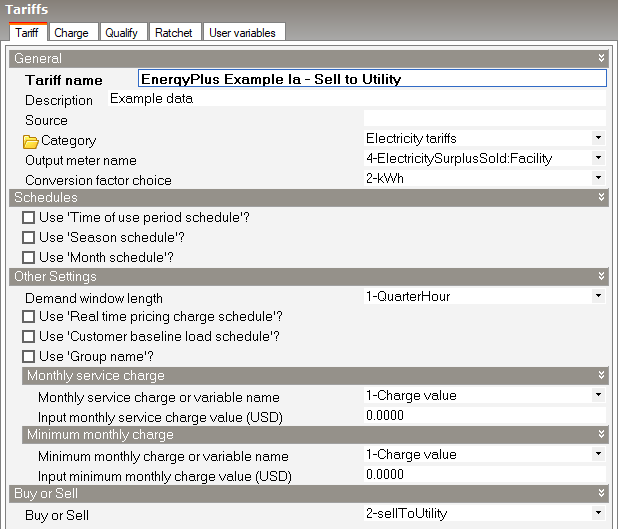
3. On the Charge tab:
Set the Number of charges to 1.
Under the Charge 1 settings header:
Set Simple or Block? to 1-Simple.
Set Charge variable name to GeneratedElectricSold
Set Source variable to totalEnergy
Set Season to 1-Annual
Set Category variable name to 1-EnergyCharges
Set Use value or variable name to 1-Value
Set Input cost per unit value to -0.020
The Charge tab should now look like the screenshot below.
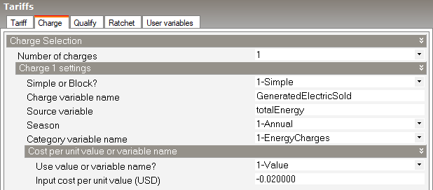
Press OK to save the Tariff data and close the dialog.
The next step is to define a rate for buying electricity and a new Tariff component needs to be created for this.
4. On the Economics model data tab, set the Number of tariffs to 2.
5. Create a second Tariff component and name it: "EnergyPlus Example Ia - Buy from Utility".
6. Open the second Tariff in the Tariff dialog and on the Tariff tab of the Tariff dialog, set the fixed monthly fee to $2.51 per month using the Input monthly service charge value setting as shown below:
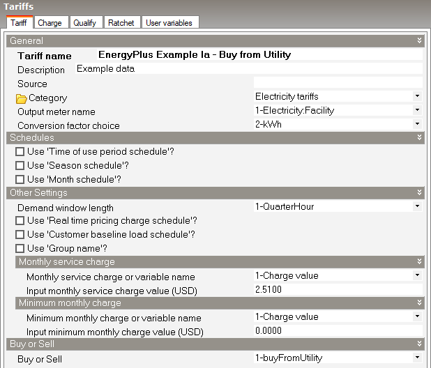
7. On the Charge tab:
Set the Number of charges to 1.
Under the Charge 1 settings header:
Set Simple or Block? to 1-Simple.
Set the Input cost per unit value to 0.055342 USD:
The Charge tab should now look like the screenshot below.
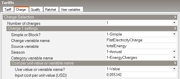
The screenshot below shows how the Economics tab should look with both Tariffs set up:
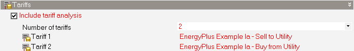
Report: Economics Results Summary Report
For: Entire Facility
Timestamp: 2025-09-11 13:02:57
Annual Cost
| Electricity | Natural Gas | Other | Total | |
| Cost [$] | 958.97 | 0.00 | 0.00 | 958.97 |
| Cost per Total Building Area [$/m2] | 5.25 | 0.00 | 0.00 | 5.25 |
| Cost per Net Conditioned Building Area [$/m2] | 5.25 | 0.00 | 0.00 | 5.25 |
Tariff Summary
| Selected | Qualified | Meter | Buy or Sell | Group | Annual Cost ($) | |
| ENERGYPLUS EXAMPLE IA - SELL TO UTILITY | Yes | Yes | ELECTRICITYSURPLUSSOLD:FACILITY | Sell | (none) | -22.0 |
| ENERGYPLUS EXAMPLE IA - BUY FROM UTILITY | Yes | Yes | ELECTRICITY:FACILITY | Buy | (none) | 981.00 |
Report: Tariff Report
For: ENERGYPLUS EXAMPLE IA - SELL TO UTILITY
Timestamp: 2025-09-11 13:02:57
General
| Parameter | |
| Meter | ELECTRICITYSURPLUSSOLD:FACILITY |
| Selected | Yes |
| Group | (none) |
| Qualified | Yes |
| Disqualifier | n/a |
| Computation | automatic |
| Units | kWh |
Categories
| Jan | Feb | Mar | Apr | May | Jun | Jul | Aug | Sep | Oct | Nov | Dec | Sum | Max | |
| EnergyCharges ($) | -0.9 | -0.6 | -2.1 | -2.2 | -2.4 | -3.6 | -3.1 | -3.2 | -1.9 | -0.9 | -0.7 | -0.3 | -22.0 | -0.3 |
| DemandCharges ($) | 0.00 | 0.00 | 0.00 | 0.00 | 0.00 | 0.00 | 0.00 | 0.00 | 0.00 | 0.00 | 0.00 | 0.00 | 0.00 | 0.00 |
| ServiceCharges ($) | 0.00 | 0.00 | 0.00 | 0.00 | 0.00 | 0.00 | 0.00 | 0.00 | 0.00 | 0.00 | 0.00 | 0.00 | 0.00 | 0.00 |
| Basis ($) | -0.9 | -0.6 | -2.1 | -2.2 | -2.4 | -3.6 | -3.1 | -3.2 | -1.9 | -0.9 | -0.7 | -0.3 | -22.0 | -0.3 |
| Adjustment ($) | 0.00 | 0.00 | 0.00 | 0.00 | 0.00 | 0.00 | 0.00 | 0.00 | 0.00 | 0.00 | 0.00 | 0.00 | 0.00 | 0.00 |
| Surcharge ($) | 0.00 | 0.00 | 0.00 | 0.00 | 0.00 | 0.00 | 0.00 | 0.00 | 0.00 | 0.00 | 0.00 | 0.00 | 0.00 | 0.00 |
| Subtotal ($) | -0.9 | -0.6 | -2.1 | -2.2 | -2.4 | -3.6 | -3.1 | -3.2 | -1.9 | -0.9 | -0.7 | -0.3 | -22.0 | -0.3 |
| Taxes ($) | 0.00 | 0.00 | 0.00 | 0.00 | 0.00 | 0.00 | 0.00 | 0.00 | 0.00 | 0.00 | 0.00 | 0.00 | 0.00 | 0.00 |
| Total ($) | -0.9 | -0.6 | -2.1 | -2.2 | -2.4 | -3.6 | -3.1 | -3.2 | -1.9 | -0.9 | -0.7 | -0.3 | -22.0 | -0.3 |
Charges
| Jan | Feb | Mar | Apr | May | Jun | Jul | Aug | Sep | Oct | Nov | Dec | Sum | Max | Category | |
| GENERATEDELECTRICSOLD ($) | -0.9 | -0.6 | -2.1 | -2.2 | -2.4 | -3.6 | -3.1 | -3.2 | -1.9 | -0.9 | -0.7 | -0.3 | -22.0 | -0.3 | EnergyCharges |
Corresponding Sources for Charges
| Jan | Feb | Mar | Apr | May | Jun | Jul | Aug | Sep | Oct | Nov | Dec | Sum | Max | |
| TotalEnergy | 46.07 | 27.70 | 103.93 | 109.71 | 121.09 | 181.01 | 156.95 | 161.28 | 96.68 | 45.64 | 35.82 | 15.70 | 1101.58 | 181.01 |
Ratchets
| Jan | Feb | Mar | Apr | May | Jun | Jul | Aug | Sep | Oct | Nov | Dec | Sum | Max |
Qualifies
| Jan | Feb | Mar | Apr | May | Jun | Jul | Aug | Sep | Oct | Nov | Dec | Sum | Max |
Native Variables
| Jan | Feb | Mar | Apr | May | Jun | Jul | Aug | Sep | Oct | Nov | Dec | Sum | Max | |
| TotalEnergy | 46.07 | 27.70 | 103.93 | 109.71 | 121.09 | 181.01 | 156.95 | 161.28 | 96.68 | 45.64 | 35.82 | 15.70 | 1101.58 | 181.01 |
| TotalDemand | 2.51 | 2.91 | 3.50 | 3.76 | 3.73 | 3.68 | 3.68 | 3.68 | 3.56 | 3.17 | 2.29 | 1.75 | 38.21 | 3.76 |
| PeakEnergy | 46.07 | 27.70 | 103.93 | 109.71 | 121.09 | 181.01 | 156.95 | 161.28 | 96.68 | 45.64 | 35.82 | 15.70 | 1101.58 | 181.01 |
| PeakDemand | 2.51 | 2.91 | 3.50 | 3.76 | 3.73 | 3.68 | 3.68 | 3.68 | 3.56 | 3.17 | 2.29 | 1.75 | 38.21 | 3.76 |
| ShoulderEnergy | 0.00 | 0.00 | 0.00 | 0.00 | 0.00 | 0.00 | 0.00 | 0.00 | 0.00 | 0.00 | 0.00 | 0.00 | 0.00 | 0.00 |
| ShoulderDemand | 0.00 | 0.00 | 0.00 | 0.00 | 0.00 | 0.00 | 0.00 | 0.00 | 0.00 | 0.00 | 0.00 | 0.00 | 0.00 | 0.00 |
| OffPeakEnergy | 0.00 | 0.00 | 0.00 | 0.00 | 0.00 | 0.00 | 0.00 | 0.00 | 0.00 | 0.00 | 0.00 | 0.00 | 0.00 | 0.00 |
| OffPeakDemand | 0.00 | 0.00 | 0.00 | 0.00 | 0.00 | 0.00 | 0.00 | 0.00 | 0.00 | 0.00 | 0.00 | 0.00 | 0.00 | 0.00 |
| MidPeakEnergy | 0.00 | 0.00 | 0.00 | 0.00 | 0.00 | 0.00 | 0.00 | 0.00 | 0.00 | 0.00 | 0.00 | 0.00 | 0.00 | 0.00 |
| MidPeakDemand | 0.00 | 0.00 | 0.00 | 0.00 | 0.00 | 0.00 | 0.00 | 0.00 | 0.00 | 0.00 | 0.00 | 0.00 | 0.00 | 0.00 |
| PeakExceedsOffPeak | 2.51 | 2.91 | 3.50 | 3.76 | 3.73 | 3.68 | 3.68 | 3.68 | 3.56 | 3.17 | 2.29 | 1.75 | 38.21 | 3.76 |
| OffPeakExceedsPeak | 0.00 | 0.00 | 0.00 | 0.00 | 0.00 | 0.00 | 0.00 | 0.00 | 0.00 | 0.00 | 0.00 | 0.00 | 0.00 | 0.00 |
| PeakExceedsMidPeak | 2.51 | 2.91 | 3.50 | 3.76 | 3.73 | 3.68 | 3.68 | 3.68 | 3.56 | 3.17 | 2.29 | 1.75 | 38.21 | 3.76 |
| MidPeakExceedsPeak | 0.00 | 0.00 | 0.00 | 0.00 | 0.00 | 0.00 | 0.00 | 0.00 | 0.00 | 0.00 | 0.00 | 0.00 | 0.00 | 0.00 |
| PeakExceedsShoulder | 2.51 | 2.91 | 3.50 | 3.76 | 3.73 | 3.68 | 3.68 | 3.68 | 3.56 | 3.17 | 2.29 | 1.75 | 38.21 | 3.76 |
| ShoulderExceedsPeak | 0.00 | 0.00 | 0.00 | 0.00 | 0.00 | 0.00 | 0.00 | 0.00 | 0.00 | 0.00 | 0.00 | 0.00 | 0.00 | 0.00 |
| IsWinter | 1.00 | 1.00 | 1.00 | 1.00 | 1.00 | 1.00 | 1.00 | 1.00 | 1.00 | 1.00 | 1.00 | 1.00 | 12.00 | 1.00 |
| IsNotWinter | 0.00 | 0.00 | 0.00 | 0.00 | 0.00 | 0.00 | 0.00 | 0.00 | 0.00 | 0.00 | 0.00 | 0.00 | 0.00 | 0.00 |
| IsSpring | 0.00 | 0.00 | 0.00 | 0.00 | 0.00 | 0.00 | 0.00 | 0.00 | 0.00 | 0.00 | 0.00 | 0.00 | 0.00 | 0.00 |
| IsNotSpring | 1.00 | 1.00 | 1.00 | 1.00 | 1.00 | 1.00 | 1.00 | 1.00 | 1.00 | 1.00 | 1.00 | 1.00 | 12.00 | 1.00 |
| IsSummer | 0.00 | 0.00 | 0.00 | 0.00 | 0.00 | 0.00 | 0.00 | 0.00 | 0.00 | 0.00 | 0.00 | 0.00 | 0.00 | 0.00 |
| IsNotSummer | 1.00 | 1.00 | 1.00 | 1.00 | 1.00 | 1.00 | 1.00 | 1.00 | 1.00 | 1.00 | 1.00 | 1.00 | 12.00 | 1.00 |
| IsAutumn | 0.00 | 0.00 | 0.00 | 0.00 | 0.00 | 0.00 | 0.00 | 0.00 | 0.00 | 0.00 | 0.00 | 0.00 | 0.00 | 0.00 |
| IsNotAutumn | 1.00 | 1.00 | 1.00 | 1.00 | 1.00 | 1.00 | 1.00 | 1.00 | 1.00 | 1.00 | 1.00 | 1.00 | 12.00 | 1.00 |
| PeakAndShoulderEnergy | 46.07 | 27.70 | 103.93 | 109.71 | 121.09 | 181.01 | 156.95 | 161.28 | 96.68 | 45.64 | 35.82 | 15.70 | 1101.58 | 181.01 |
| PeakAndShoulderDemand | 2.51 | 2.91 | 3.50 | 3.76 | 3.73 | 3.68 | 3.68 | 3.68 | 3.56 | 3.17 | 2.29 | 1.75 | 38.21 | 3.76 |
| PeakAndMidPeakEnergy | 46.07 | 27.70 | 103.93 | 109.71 | 121.09 | 181.01 | 156.95 | 161.28 | 96.68 | 45.64 | 35.82 | 15.70 | 1101.58 | 181.01 |
| PeakAndMidPeakDemand | 2.51 | 2.91 | 3.50 | 3.76 | 3.73 | 3.68 | 3.68 | 3.68 | 3.56 | 3.17 | 2.29 | 1.75 | 38.21 | 3.76 |
| ShoulderAndOffPeakEnergy | 0.00 | 0.00 | 0.00 | 0.00 | 0.00 | 0.00 | 0.00 | 0.00 | 0.00 | 0.00 | 0.00 | 0.00 | 0.00 | 0.00 |
| ShoulderAndOffPeakDemand | 0.00 | 0.00 | 0.00 | 0.00 | 0.00 | 0.00 | 0.00 | 0.00 | 0.00 | 0.00 | 0.00 | 0.00 | 0.00 | 0.00 |
| PeakAndOffPeakEnergy | 46.07 | 27.70 | 103.93 | 109.71 | 121.09 | 181.01 | 156.95 | 161.28 | 96.68 | 45.64 | 35.82 | 15.70 | 1101.58 | 181.01 |
| PeakAndOffPeakDemand | 2.51 | 2.91 | 3.50 | 3.76 | 3.73 | 3.68 | 3.68 | 3.68 | 3.56 | 3.17 | 2.29 | 1.75 | 38.21 | 3.76 |
| RealTimePriceCosts | 0.00 | 0.00 | 0.00 | 0.00 | 0.00 | 0.00 | 0.00 | 0.00 | 0.00 | 0.00 | 0.00 | 0.00 | 0.00 | 0.00 |
| AboveCustomerBaseCosts | 0.00 | 0.00 | 0.00 | 0.00 | 0.00 | 0.00 | 0.00 | 0.00 | 0.00 | 0.00 | 0.00 | 0.00 | 0.00 | 0.00 |
| BelowCustomerBaseCosts | 0.00 | 0.00 | 0.00 | 0.00 | 0.00 | 0.00 | 0.00 | 0.00 | 0.00 | 0.00 | 0.00 | 0.00 | 0.00 | 0.00 |
| AboveCustomerBaseEnergy | 0.00 | 0.00 | 0.00 | 0.00 | 0.00 | 0.00 | 0.00 | 0.00 | 0.00 | 0.00 | 0.00 | 0.00 | 0.00 | 0.00 |
| BelowCustomerBaseEnergy | 0.00 | 0.00 | 0.00 | 0.00 | 0.00 | 0.00 | 0.00 | 0.00 | 0.00 | 0.00 | 0.00 | 0.00 | 0.00 | 0.00 |
Other Variables
| Jan | Feb | Mar | Apr | May | Jun | Jul | Aug | Sep | Oct | Nov | Dec | Sum | Max | |
| NotIncluded | 0.00 | 0.00 | 0.00 | 0.00 | 0.00 | 0.00 | 0.00 | 0.00 | 0.00 | 0.00 | 0.00 | 0.00 | 0.00 | 0.00 |
Report: Tariff Report
For: ENERGYPLUS EXAMPLE IA - BUY FROM UTILITY
Timestamp: 2025-09-11 13:02:57
General
| Parameter | |
| Meter | ELECTRICITY:FACILITY |
| Selected | Yes |
| Group | (none) |
| Qualified | Yes |
| Disqualifier | n/a |
| Computation | automatic |
| Units | kWh |
Categories
| Jan | Feb | Mar | Apr | May | Jun | Jul | Aug | Sep | Oct | Nov | Dec | Sum | Max | |
| EnergyCharges ($) | 69.81 | 61.60 | 67.17 | 79.44 | 93.88 | 84.38 | 102.56 | 95.86 | 83.67 | 79.83 | 65.44 | 67.24 | 950.88 | 102.56 |
| DemandCharges ($) | 0.00 | 0.00 | 0.00 | 0.00 | 0.00 | 0.00 | 0.00 | 0.00 | 0.00 | 0.00 | 0.00 | 0.00 | 0.00 | 0.00 |
| ServiceCharges ($) | 2.51 | 2.51 | 2.51 | 2.51 | 2.51 | 2.51 | 2.51 | 2.51 | 2.51 | 2.51 | 2.51 | 2.51 | 30.12 | 2.51 |
| Basis ($) | 72.32 | 64.11 | 69.68 | 81.95 | 96.39 | 86.89 | 105.07 | 98.37 | 86.18 | 82.34 | 67.95 | 69.75 | 981.00 | 105.07 |
| Adjustment ($) | 0.00 | 0.00 | 0.00 | 0.00 | 0.00 | 0.00 | 0.00 | 0.00 | 0.00 | 0.00 | 0.00 | 0.00 | 0.00 | 0.00 |
| Surcharge ($) | 0.00 | 0.00 | 0.00 | 0.00 | 0.00 | 0.00 | 0.00 | 0.00 | 0.00 | 0.00 | 0.00 | 0.00 | 0.00 | 0.00 |
| Subtotal ($) | 72.32 | 64.11 | 69.68 | 81.95 | 96.39 | 86.89 | 105.07 | 98.37 | 86.18 | 82.34 | 67.95 | 69.75 | 981.00 | 105.07 |
| Taxes ($) | 0.00 | 0.00 | 0.00 | 0.00 | 0.00 | 0.00 | 0.00 | 0.00 | 0.00 | 0.00 | 0.00 | 0.00 | 0.00 | 0.00 |
| Total ($) | 72.32 | 64.11 | 69.68 | 81.95 | 96.39 | 86.89 | 105.07 | 98.37 | 86.18 | 82.34 | 67.95 | 69.75 | 981.00 | 105.07 |
Charges
| Jan | Feb | Mar | Apr | May | Jun | Jul | Aug | Sep | Oct | Nov | Dec | Sum | Max | Category | |
| FLATELECTRICITYCHARGE ($) | 69.81 | 61.60 | 67.17 | 79.44 | 93.88 | 84.38 | 102.56 | 95.86 | 83.67 | 79.83 | 65.44 | 67.24 | 950.88 | 102.56 | EnergyCharges |
Corresponding Sources for Charges
| Jan | Feb | Mar | Apr | May | Jun | Jul | Aug | Sep | Oct | Nov | Dec | Sum | Max | |
| TotalEnergy | 1261.35 | 1113.04 | 1213.71 | 1435.50 | 1696.34 | 1524.70 | 1853.15 | 1732.16 | 1511.94 | 1442.50 | 1182.46 | 1215.03 | 17181.89 | 1853.15 |
Ratchets
| Jan | Feb | Mar | Apr | May | Jun | Jul | Aug | Sep | Oct | Nov | Dec | Sum | Max |
Qualifies
| Jan | Feb | Mar | Apr | May | Jun | Jul | Aug | Sep | Oct | Nov | Dec | Sum | Max |
Native Variables
| Jan | Feb | Mar | Apr | May | Jun | Jul | Aug | Sep | Oct | Nov | Dec | Sum | Max | |
| TotalEnergy | 1261.35 | 1113.04 | 1213.71 | 1435.50 | 1696.34 | 1524.70 | 1853.15 | 1732.16 | 1511.94 | 1442.50 | 1182.46 | 1215.03 | 17181.89 | 1853.15 |
| TotalDemand | 4.07 | 5.39 | 5.82 | 6.17 | 6.77 | 7.55 | 7.63 | 7.96 | 6.67 | 6.12 | 5.64 | 4.07 | 73.85 | 7.96 |
| PeakEnergy | 1261.35 | 1113.04 | 1213.71 | 1435.50 | 1696.34 | 1524.70 | 1853.15 | 1732.16 | 1511.94 | 1442.50 | 1182.46 | 1215.03 | 17181.89 | 1853.15 |
| PeakDemand | 4.07 | 5.39 | 5.82 | 6.17 | 6.77 | 7.55 | 7.63 | 7.96 | 6.67 | 6.12 | 5.64 | 4.07 | 73.85 | 7.96 |
| ShoulderEnergy | 0.00 | 0.00 | 0.00 | 0.00 | 0.00 | 0.00 | 0.00 | 0.00 | 0.00 | 0.00 | 0.00 | 0.00 | 0.00 | 0.00 |
| ShoulderDemand | 0.00 | 0.00 | 0.00 | 0.00 | 0.00 | 0.00 | 0.00 | 0.00 | 0.00 | 0.00 | 0.00 | 0.00 | 0.00 | 0.00 |
| OffPeakEnergy | 0.00 | 0.00 | 0.00 | 0.00 | 0.00 | 0.00 | 0.00 | 0.00 | 0.00 | 0.00 | 0.00 | 0.00 | 0.00 | 0.00 |
| OffPeakDemand | 0.00 | 0.00 | 0.00 | 0.00 | 0.00 | 0.00 | 0.00 | 0.00 | 0.00 | 0.00 | 0.00 | 0.00 | 0.00 | 0.00 |
| MidPeakEnergy | 0.00 | 0.00 | 0.00 | 0.00 | 0.00 | 0.00 | 0.00 | 0.00 | 0.00 | 0.00 | 0.00 | 0.00 | 0.00 | 0.00 |
| MidPeakDemand | 0.00 | 0.00 | 0.00 | 0.00 | 0.00 | 0.00 | 0.00 | 0.00 | 0.00 | 0.00 | 0.00 | 0.00 | 0.00 | 0.00 |
| PeakExceedsOffPeak | 4.07 | 5.39 | 5.82 | 6.17 | 6.77 | 7.55 | 7.63 | 7.96 | 6.67 | 6.12 | 5.64 | 4.07 | 73.85 | 7.96 |
| OffPeakExceedsPeak | 0.00 | 0.00 | 0.00 | 0.00 | 0.00 | 0.00 | 0.00 | 0.00 | 0.00 | 0.00 | 0.00 | 0.00 | 0.00 | 0.00 |
| PeakExceedsMidPeak | 4.07 | 5.39 | 5.82 | 6.17 | 6.77 | 7.55 | 7.63 | 7.96 | 6.67 | 6.12 | 5.64 | 4.07 | 73.85 | 7.96 |
| MidPeakExceedsPeak | 0.00 | 0.00 | 0.00 | 0.00 | 0.00 | 0.00 | 0.00 | 0.00 | 0.00 | 0.00 | 0.00 | 0.00 | 0.00 | 0.00 |
| PeakExceedsShoulder | 4.07 | 5.39 | 5.82 | 6.17 | 6.77 | 7.55 | 7.63 | 7.96 | 6.67 | 6.12 | 5.64 | 4.07 | 73.85 | 7.96 |
| ShoulderExceedsPeak | 0.00 | 0.00 | 0.00 | 0.00 | 0.00 | 0.00 | 0.00 | 0.00 | 0.00 | 0.00 | 0.00 | 0.00 | 0.00 | 0.00 |
| IsWinter | 1.00 | 1.00 | 1.00 | 1.00 | 1.00 | 1.00 | 1.00 | 1.00 | 1.00 | 1.00 | 1.00 | 1.00 | 12.00 | 1.00 |
| IsNotWinter | 0.00 | 0.00 | 0.00 | 0.00 | 0.00 | 0.00 | 0.00 | 0.00 | 0.00 | 0.00 | 0.00 | 0.00 | 0.00 | 0.00 |
| IsSpring | 0.00 | 0.00 | 0.00 | 0.00 | 0.00 | 0.00 | 0.00 | 0.00 | 0.00 | 0.00 | 0.00 | 0.00 | 0.00 | 0.00 |
| IsNotSpring | 1.00 | 1.00 | 1.00 | 1.00 | 1.00 | 1.00 | 1.00 | 1.00 | 1.00 | 1.00 | 1.00 | 1.00 | 12.00 | 1.00 |
| IsSummer | 0.00 | 0.00 | 0.00 | 0.00 | 0.00 | 0.00 | 0.00 | 0.00 | 0.00 | 0.00 | 0.00 | 0.00 | 0.00 | 0.00 |
| IsNotSummer | 1.00 | 1.00 | 1.00 | 1.00 | 1.00 | 1.00 | 1.00 | 1.00 | 1.00 | 1.00 | 1.00 | 1.00 | 12.00 | 1.00 |
| IsAutumn | 0.00 | 0.00 | 0.00 | 0.00 | 0.00 | 0.00 | 0.00 | 0.00 | 0.00 | 0.00 | 0.00 | 0.00 | 0.00 | 0.00 |
| IsNotAutumn | 1.00 | 1.00 | 1.00 | 1.00 | 1.00 | 1.00 | 1.00 | 1.00 | 1.00 | 1.00 | 1.00 | 1.00 | 12.00 | 1.00 |
| PeakAndShoulderEnergy | 1261.35 | 1113.04 | 1213.71 | 1435.50 | 1696.34 | 1524.70 | 1853.15 | 1732.16 | 1511.94 | 1442.50 | 1182.46 | 1215.03 | 17181.89 | 1853.15 |
| PeakAndShoulderDemand | 4.07 | 5.39 | 5.82 | 6.17 | 6.77 | 7.55 | 7.63 | 7.96 | 6.67 | 6.12 | 5.64 | 4.07 | 73.85 | 7.96 |
| PeakAndMidPeakEnergy | 1261.35 | 1113.04 | 1213.71 | 1435.50 | 1696.34 | 1524.70 | 1853.15 | 1732.16 | 1511.94 | 1442.50 | 1182.46 | 1215.03 | 17181.89 | 1853.15 |
| PeakAndMidPeakDemand | 4.07 | 5.39 | 5.82 | 6.17 | 6.77 | 7.55 | 7.63 | 7.96 | 6.67 | 6.12 | 5.64 | 4.07 | 73.85 | 7.96 |
| ShoulderAndOffPeakEnergy | 0.00 | 0.00 | 0.00 | 0.00 | 0.00 | 0.00 | 0.00 | 0.00 | 0.00 | 0.00 | 0.00 | 0.00 | 0.00 | 0.00 |
| ShoulderAndOffPeakDemand | 0.00 | 0.00 | 0.00 | 0.00 | 0.00 | 0.00 | 0.00 | 0.00 | 0.00 | 0.00 | 0.00 | 0.00 | 0.00 | 0.00 |
| PeakAndOffPeakEnergy | 1261.35 | 1113.04 | 1213.71 | 1435.50 | 1696.34 | 1524.70 | 1853.15 | 1732.16 | 1511.94 | 1442.50 | 1182.46 | 1215.03 | 17181.89 | 1853.15 |
| PeakAndOffPeakDemand | 4.07 | 5.39 | 5.82 | 6.17 | 6.77 | 7.55 | 7.63 | 7.96 | 6.67 | 6.12 | 5.64 | 4.07 | 73.85 | 7.96 |
| RealTimePriceCosts | 0.00 | 0.00 | 0.00 | 0.00 | 0.00 | 0.00 | 0.00 | 0.00 | 0.00 | 0.00 | 0.00 | 0.00 | 0.00 | 0.00 |
| AboveCustomerBaseCosts | 0.00 | 0.00 | 0.00 | 0.00 | 0.00 | 0.00 | 0.00 | 0.00 | 0.00 | 0.00 | 0.00 | 0.00 | 0.00 | 0.00 |
| BelowCustomerBaseCosts | 0.00 | 0.00 | 0.00 | 0.00 | 0.00 | 0.00 | 0.00 | 0.00 | 0.00 | 0.00 | 0.00 | 0.00 | 0.00 | 0.00 |
| AboveCustomerBaseEnergy | 0.00 | 0.00 | 0.00 | 0.00 | 0.00 | 0.00 | 0.00 | 0.00 | 0.00 | 0.00 | 0.00 | 0.00 | 0.00 | 0.00 |
| BelowCustomerBaseEnergy | 0.00 | 0.00 | 0.00 | 0.00 | 0.00 | 0.00 | 0.00 | 0.00 | 0.00 | 0.00 | 0.00 | 0.00 | 0.00 | 0.00 |
In this example, a "net-metering" tariff is defined with the Buy or Sell field set to 3-netMetering, and the Output meter set to 5-ElectricityNet:Facility. The Tariff is set up as follows:
Customer charge: $30 per month
Net metering charge: 6.5 cents/kWh
To create this tariff, follow the steps below.
1. On the Economics model data tab, set the Number of tariffs to 1.
2. Create a new Tariff component and name it: "EnergyPlus Example Ib - Net-Metering"
The screenshot below shows how the Economics tab should now look with the Tariff set up:
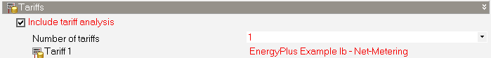
5. Open the Tariff component in the Tariff dialog and on the Tariff tab:
Set the Output meter name to 5-ElectricityNet:Facility
Set the fixed monthly fee to $30 per month using the Input monthly service charge value setting.
Set Buy or Sell to 3-netMetering
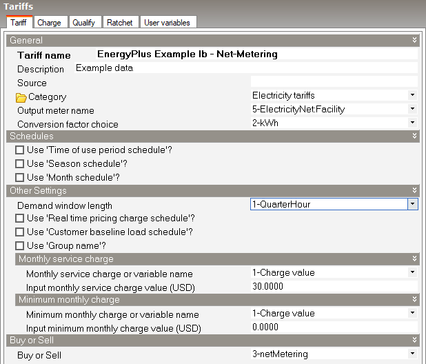
6. On the Charge tab:
Set the Number of charges to 1.
Under the Charge 1 settings header:
Set Simple or Block? to 1-Simple.
Set Charge variable name to NetMeteredCharge
Set Source variable to totalEnergy
Set Season to 1-Annual
Set Category variable name to 1-EnergyCharges
Set Use value or variable name to 1-Value
Set Input cost per unit value to 0.0650
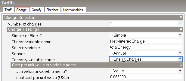
Report: Economics Results Summary Report
For: Entire Facility
Timestamp: 2025-09-11 13:09:35
Annual Cost
| Electricity | Natural Gas | Other | Total | |
| Cost [$] | 1182.21 | 0.00 | 0.00 | 1182.21 |
| Cost per Total Building Area [$/m2] | 6.47 | 0.00 | 0.00 | 6.47 |
| Cost per Net Conditioned Building Area [$/m2] | 6.47 | 0.00 | 0.00 | 6.47 |
Tariff Summary
| Selected | Qualified | Meter | Buy or Sell | Group | Annual Cost ($) | |
| ENERGYPLUS EXAMPLE IB - NET-METERING | Yes | Yes | ELECTRICITYNET:FACILITY | Net | (none) | 1182.21 |
Report: Tariff Report
For: ENERGYPLUS EXAMPLE IB - NET-METERING
Timestamp: 2025-09-11 13:09:35
General
| Parameter | |
| Meter | ELECTRICITYNET:FACILITY |
| Selected | Yes |
| Group | (none) |
| Qualified | Yes |
| Disqualifier | n/a |
| Computation | automatic |
| Units | kWh |
Categories
| Jan | Feb | Mar | Apr | May | Jun | Jul | Aug | Sep | Oct | Nov | Dec | Sum | Max | |
| EnergyCharges ($) | 71.19 | 59.18 | 58.26 | 61.66 | 71.65 | 63.27 | 81.46 | 75.34 | 70.58 | 73.19 | 64.89 | 71.55 | 822.21 | 81.46 |
| DemandCharges ($) | 0.00 | 0.00 | 0.00 | 0.00 | 0.00 | 0.00 | 0.00 | 0.00 | 0.00 | 0.00 | 0.00 | 0.00 | 0.00 | 0.00 |
| ServiceCharges ($) | 30.00 | 30.00 | 30.00 | 30.00 | 30.00 | 30.00 | 30.00 | 30.00 | 30.00 | 30.00 | 30.00 | 30.00 | 360.00 | 30.00 |
| Basis ($) | 101.19 | 89.18 | 88.26 | 91.66 | 101.65 | 93.27 | 111.46 | 105.34 | 100.58 | 103.19 | 94.89 | 101.55 | 1182.21 | 111.46 |
| Adjustment ($) | 0.00 | 0.00 | 0.00 | 0.00 | 0.00 | 0.00 | 0.00 | 0.00 | 0.00 | 0.00 | 0.00 | 0.00 | 0.00 | 0.00 |
| Surcharge ($) | 0.00 | 0.00 | 0.00 | 0.00 | 0.00 | 0.00 | 0.00 | 0.00 | 0.00 | 0.00 | 0.00 | 0.00 | 0.00 | 0.00 |
| Subtotal ($) | 101.19 | 89.18 | 88.26 | 91.66 | 101.65 | 93.27 | 111.46 | 105.34 | 100.58 | 103.19 | 94.89 | 101.55 | 1182.21 | 111.46 |
| Taxes ($) | 0.00 | 0.00 | 0.00 | 0.00 | 0.00 | 0.00 | 0.00 | 0.00 | 0.00 | 0.00 | 0.00 | 0.00 | 0.00 | 0.00 |
| Total ($) | 101.19 | 89.18 | 88.26 | 91.66 | 101.65 | 93.27 | 111.46 | 105.34 | 100.58 | 103.19 | 94.89 | 101.55 | 1182.21 | 111.46 |
Charges
| Jan | Feb | Mar | Apr | May | Jun | Jul | Aug | Sep | Oct | Nov | Dec | Sum | Max | Category | |
| NETMETEREDCHARGE ($) | 71.19 | 59.18 | 58.26 | 61.66 | 71.65 | 63.27 | 81.46 | 75.34 | 70.58 | 73.19 | 64.89 | 71.55 | 822.21 | 81.46 | EnergyCharges |
Corresponding Sources for Charges
| Jan | Feb | Mar | Apr | May | Jun | Jul | Aug | Sep | Oct | Nov | Dec | Sum | Max | |
| TotalEnergy | 1095.29 | 910.42 | 896.28 | 948.56 | 1102.25 | 973.35 | 1253.20 | 1159.11 | 1085.83 | 1125.98 | 998.29 | 1100.84 | 12649.40 | 1253.20 |
Ratchets
| Jan | Feb | Mar | Apr | May | Jun | Jul | Aug | Sep | Oct | Nov | Dec | Sum | Max |
Qualifies
| Jan | Feb | Mar | Apr | May | Jun | Jul | Aug | Sep | Oct | Nov | Dec | Sum | Max |
Native Variables
| Jan | Feb | Mar | Apr | May | Jun | Jul | Aug | Sep | Oct | Nov | Dec | Sum | Max | |
| TotalEnergy | 1095.29 | 910.42 | 896.28 | 948.56 | 1102.25 | 973.35 | 1253.20 | 1159.11 | 1085.83 | 1125.98 | 998.29 | 1100.84 | 12649.40 | 1253.20 |
| TotalDemand | 4.07 | 4.06 | 5.21 | 5.55 | 5.83 | 6.10 | 6.14 | 6.39 | 5.85 | 5.65 | 5.08 | 4.07 | 64.01 | 6.39 |
| PeakEnergy | 1095.29 | 910.42 | 896.28 | 948.56 | 1102.25 | 973.35 | 1253.20 | 1159.11 | 1085.83 | 1125.98 | 998.29 | 1100.84 | 12649.40 | 1253.20 |
| PeakDemand | 4.07 | 4.06 | 5.21 | 5.55 | 5.83 | 6.10 | 6.14 | 6.39 | 5.85 | 5.65 | 5.08 | 4.07 | 64.01 | 6.39 |
| ShoulderEnergy | 0.00 | 0.00 | 0.00 | 0.00 | 0.00 | 0.00 | 0.00 | 0.00 | 0.00 | 0.00 | 0.00 | 0.00 | 0.00 | 0.00 |
| ShoulderDemand | 0.00 | 0.00 | 0.00 | 0.00 | 0.00 | 0.00 | 0.00 | 0.00 | 0.00 | 0.00 | 0.00 | 0.00 | 0.00 | 0.00 |
| OffPeakEnergy | 0.00 | 0.00 | 0.00 | 0.00 | 0.00 | 0.00 | 0.00 | 0.00 | 0.00 | 0.00 | 0.00 | 0.00 | 0.00 | 0.00 |
| OffPeakDemand | 0.00 | 0.00 | 0.00 | 0.00 | 0.00 | 0.00 | 0.00 | 0.00 | 0.00 | 0.00 | 0.00 | 0.00 | 0.00 | 0.00 |
| MidPeakEnergy | 0.00 | 0.00 | 0.00 | 0.00 | 0.00 | 0.00 | 0.00 | 0.00 | 0.00 | 0.00 | 0.00 | 0.00 | 0.00 | 0.00 |
| MidPeakDemand | 0.00 | 0.00 | 0.00 | 0.00 | 0.00 | 0.00 | 0.00 | 0.00 | 0.00 | 0.00 | 0.00 | 0.00 | 0.00 | 0.00 |
| PeakExceedsOffPeak | 4.07 | 4.06 | 5.21 | 5.55 | 5.83 | 6.10 | 6.14 | 6.39 | 5.85 | 5.65 | 5.08 | 4.07 | 64.01 | 6.39 |
| OffPeakExceedsPeak | 0.00 | 0.00 | 0.00 | 0.00 | 0.00 | 0.00 | 0.00 | 0.00 | 0.00 | 0.00 | 0.00 | 0.00 | 0.00 | 0.00 |
| PeakExceedsMidPeak | 4.07 | 4.06 | 5.21 | 5.55 | 5.83 | 6.10 | 6.14 | 6.39 | 5.85 | 5.65 | 5.08 | 4.07 | 64.01 | 6.39 |
| MidPeakExceedsPeak | 0.00 | 0.00 | 0.00 | 0.00 | 0.00 | 0.00 | 0.00 | 0.00 | 0.00 | 0.00 | 0.00 | 0.00 | 0.00 | 0.00 |
| PeakExceedsShoulder | 4.07 | 4.06 | 5.21 | 5.55 | 5.83 | 6.10 | 6.14 | 6.39 | 5.85 | 5.65 | 5.08 | 4.07 | 64.01 | 6.39 |
| ShoulderExceedsPeak | 0.00 | 0.00 | 0.00 | 0.00 | 0.00 | 0.00 | 0.00 | 0.00 | 0.00 | 0.00 | 0.00 | 0.00 | 0.00 | 0.00 |
| IsWinter | 1.00 | 1.00 | 1.00 | 1.00 | 1.00 | 1.00 | 1.00 | 1.00 | 1.00 | 1.00 | 1.00 | 1.00 | 12.00 | 1.00 |
| IsNotWinter | 0.00 | 0.00 | 0.00 | 0.00 | 0.00 | 0.00 | 0.00 | 0.00 | 0.00 | 0.00 | 0.00 | 0.00 | 0.00 | 0.00 |
| IsSpring | 0.00 | 0.00 | 0.00 | 0.00 | 0.00 | 0.00 | 0.00 | 0.00 | 0.00 | 0.00 | 0.00 | 0.00 | 0.00 | 0.00 |
| IsNotSpring | 1.00 | 1.00 | 1.00 | 1.00 | 1.00 | 1.00 | 1.00 | 1.00 | 1.00 | 1.00 | 1.00 | 1.00 | 12.00 | 1.00 |
| IsSummer | 0.00 | 0.00 | 0.00 | 0.00 | 0.00 | 0.00 | 0.00 | 0.00 | 0.00 | 0.00 | 0.00 | 0.00 | 0.00 | 0.00 |
| IsNotSummer | 1.00 | 1.00 | 1.00 | 1.00 | 1.00 | 1.00 | 1.00 | 1.00 | 1.00 | 1.00 | 1.00 | 1.00 | 12.00 | 1.00 |
| IsAutumn | 0.00 | 0.00 | 0.00 | 0.00 | 0.00 | 0.00 | 0.00 | 0.00 | 0.00 | 0.00 | 0.00 | 0.00 | 0.00 | 0.00 |
| IsNotAutumn | 1.00 | 1.00 | 1.00 | 1.00 | 1.00 | 1.00 | 1.00 | 1.00 | 1.00 | 1.00 | 1.00 | 1.00 | 12.00 | 1.00 |
| PeakAndShoulderEnergy | 1095.29 | 910.42 | 896.28 | 948.56 | 1102.25 | 973.35 | 1253.20 | 1159.11 | 1085.83 | 1125.98 | 998.29 | 1100.84 | 12649.40 | 1253.20 |
| PeakAndShoulderDemand | 4.07 | 4.06 | 5.21 | 5.55 | 5.83 | 6.10 | 6.14 | 6.39 | 5.85 | 5.65 | 5.08 | 4.07 | 64.01 | 6.39 |
| PeakAndMidPeakEnergy | 1095.29 | 910.42 | 896.28 | 948.56 | 1102.25 | 973.35 | 1253.20 | 1159.11 | 1085.83 | 1125.98 | 998.29 | 1100.84 | 12649.40 | 1253.20 |
| PeakAndMidPeakDemand | 4.07 | 4.06 | 5.21 | 5.55 | 5.83 | 6.10 | 6.14 | 6.39 | 5.85 | 5.65 | 5.08 | 4.07 | 64.01 | 6.39 |
| ShoulderAndOffPeakEnergy | 0.00 | 0.00 | 0.00 | 0.00 | 0.00 | 0.00 | 0.00 | 0.00 | 0.00 | 0.00 | 0.00 | 0.00 | 0.00 | 0.00 |
| ShoulderAndOffPeakDemand | 0.00 | 0.00 | 0.00 | 0.00 | 0.00 | 0.00 | 0.00 | 0.00 | 0.00 | 0.00 | 0.00 | 0.00 | 0.00 | 0.00 |
| PeakAndOffPeakEnergy | 1095.29 | 910.42 | 896.28 | 948.56 | 1102.25 | 973.35 | 1253.20 | 1159.11 | 1085.83 | 1125.98 | 998.29 | 1100.84 | 12649.40 | 1253.20 |
| PeakAndOffPeakDemand | 4.07 | 4.06 | 5.21 | 5.55 | 5.83 | 6.10 | 6.14 | 6.39 | 5.85 | 5.65 | 5.08 | 4.07 | 64.01 | 6.39 |
| RealTimePriceCosts | 0.00 | 0.00 | 0.00 | 0.00 | 0.00 | 0.00 | 0.00 | 0.00 | 0.00 | 0.00 | 0.00 | 0.00 | 0.00 | 0.00 |
| AboveCustomerBaseCosts | 0.00 | 0.00 | 0.00 | 0.00 | 0.00 | 0.00 | 0.00 | 0.00 | 0.00 | 0.00 | 0.00 | 0.00 | 0.00 | 0.00 |
| BelowCustomerBaseCosts | 0.00 | 0.00 | 0.00 | 0.00 | 0.00 | 0.00 | 0.00 | 0.00 | 0.00 | 0.00 | 0.00 | 0.00 | 0.00 | 0.00 |
| AboveCustomerBaseEnergy | 0.00 | 0.00 | 0.00 | 0.00 | 0.00 | 0.00 | 0.00 | 0.00 | 0.00 | 0.00 | 0.00 | 0.00 | 0.00 | 0.00 |
| BelowCustomerBaseEnergy | 0.00 | 0.00 | 0.00 | 0.00 | 0.00 | 0.00 | 0.00 | 0.00 | 0.00 | 0.00 | 0.00 | 0.00 | 0.00 | 0.00 |
This example shows how to model a dual ratchet demand structure where the billed demand is the greater of a rolling 12-month peak or a fixed minimum threshold. This approach is suitable for commercial tariffs that combine historical peak demand tracking with guaranteed minimum billing levels to ensure utility cost recovery.
Note: This example uses the GBP currency instead of USD. You can change Currency on the International tab of the Program options dialog.
Determination of Distribution Demand will be the highest of:
The highest average kW measured during any 30-minute interval of the current and previous 11 billing months (rolling 12-month peak).
A fixed minimum demand of 500 kW.
The example demonstrates two separate approaches to modelling the minimum demand:
Ratchet Multiplier and Offset: This approach uses a very small but non-zero multiplier in the UtilityCost:Ratchet object to simulate the minimum billing threshold.
Block Charge based Minimum Billing: The same minimum billing condition can be modelled directly through a UtilityCost:Charge:Block object.
Use a very small but non-zero ratchet multiplier. In this case, the offset should be set to 500 × (1 / multiplier). For example, you can use a multiplier of 0.001 and an offset of 500,000.
To create this tariff structure, starting by ensuring you have the GBP currency set in Program options and follow the steps below.
1. Create a new Tariff component:

2. On the Tariff tab of the Tariff dialog:
Set the Demand window length to 2-HalfHour to ensure correct 30-minute average interval.
The Tariff tab should now look similar to the screenshot below:
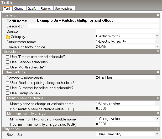
Note: The Demand window length choice may be overridden based on the value of Simulation time step so that they are consistent, i.e. demand window length should be exact multiples of the simulation time step length in minutes. For example, if the time step is 6, i.e. a 10 minutes time step, then QuarterHour is not used and instead HalfHour is used. Or if time step is 3, i.e. 20 minutes time step, then QuarterHour and HalfHour are not used and instead FullHour is used.
3. On the Ratchet tab:
Set the Number of ratchets to 2.
Under the Ratchet 1 settings header:
Set Ratchet variable name to BillingDemandA
Set Baseline source variable to TotalDemand
Set Adjustment source variable to TotalDemand
Set Season from to 1-Annual
Set Season to to 1-Annual
Under the Multiplier value or variable name header, set Use value or variable name? to 1-Value
Under the Multiplier value or variable name header, set Input multiplier value to 1
Under the Offset value or variable name header, set Use value or variable name? to 1-Value
Under the Offset value or variable name header, set Input offset value to 0
Under the Ratchet 2 settings header:
Set Ratchet variable name to BillingDemandB
Set Baseline source variable to BillingDemandA
Set Adjustment source variable to TotalDemand
Set Season from to 6-Monthly
Set Season to to 1-Annual
Under the Multiplier value or variable name header, set Use value or variable name? to 1-Value
Under the Multiplier value or variable name header, set Input multiplier value to 0.001
Under the Offset value or variable name header, set Use value or variable name? to 1-Value
Under the Offset value or variable name header, set Input offset value to 500,000
The Ratchet tab should now look similar to the screenshot below.
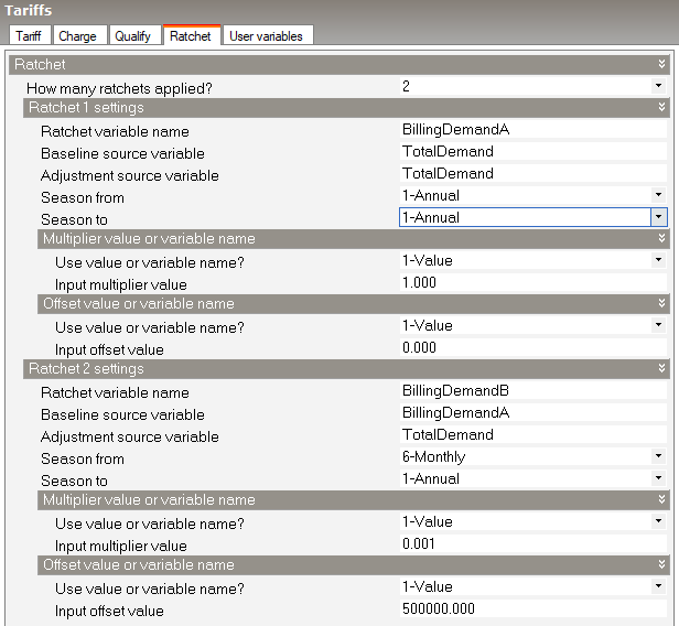
Report: Economics Results Summary Report
For: Entire Facility
Timestamp: 2025-10-17 13:27:12
Annual Cost
| Electricity | Natural Gas | Other | Total | |
| Cost [£] | 300.00 | 0.00 | 0.00 | 300.00 |
| Cost per Total Building Area [£/m2] | 1.64 | 0.00 | 0.00 | 1.64 |
| Cost per Net Conditioned Building Area [£/m2] | 1.64 | 0.00 | 0.00 | 1.64 |
Tariff Summary
| Selected | Qualified | Meter | Buy or Sell | Group | Annual Cost (£) | |
| EXAMPLE JA - RATCHET MULTIPLIER AND OFFSET | Yes | Yes | ELECTRICITY:FACILITY | Buy | (none) | 300.00 |
Report: Tariff Report
For: EXAMPLE JA - RATCHET MULTIPLIER AND OFFSET
Timestamp: 2025-10-17 13:27:12
General
| Parameter | |
| Meter | ELECTRICITY:FACILITY |
| Selected | Yes |
| Group | (none) |
| Qualified | Yes |
| Disqualifier | n/a |
| Computation | automatic |
| Units | kWh |
Categories
| Jan | Feb | Mar | Apr | May | Jun | Jul | Aug | Sep | Oct | Nov | Dec | Sum | Max | |
| EnergyCharges (£) | 0.00 | 0.00 | 0.00 | 0.00 | 0.00 | 0.00 | 0.00 | 0.00 | 0.00 | 0.00 | 0.00 | 0.00 | 0.00 | 0.00 |
| DemandCharges (£) | 25.00 | 25.00 | 25.00 | 25.00 | 25.00 | 25.00 | 25.00 | 25.00 | 25.00 | 25.00 | 25.00 | 25.00 | 300.00 | 25.00 |
| ServiceCharges (£) | 0.00 | 0.00 | 0.00 | 0.00 | 0.00 | 0.00 | 0.00 | 0.00 | 0.00 | 0.00 | 0.00 | 0.00 | 0.00 | 0.00 |
| Basis (£) | 25.00 | 25.00 | 25.00 | 25.00 | 25.00 | 25.00 | 25.00 | 25.00 | 25.00 | 25.00 | 25.00 | 25.00 | 300.00 | 25.00 |
| Adjustment (£) | 0.00 | 0.00 | 0.00 | 0.00 | 0.00 | 0.00 | 0.00 | 0.00 | 0.00 | 0.00 | 0.00 | 0.00 | 0.00 | 0.00 |
| Surcharge (£) | 0.00 | 0.00 | 0.00 | 0.00 | 0.00 | 0.00 | 0.00 | 0.00 | 0.00 | 0.00 | 0.00 | 0.00 | 0.00 | 0.00 |
| Subtotal (£) | 25.00 | 25.00 | 25.00 | 25.00 | 25.00 | 25.00 | 25.00 | 25.00 | 25.00 | 25.00 | 25.00 | 25.00 | 300.00 | 25.00 |
| Taxes (£) | 0.00 | 0.00 | 0.00 | 0.00 | 0.00 | 0.00 | 0.00 | 0.00 | 0.00 | 0.00 | 0.00 | 0.00 | 0.00 | 0.00 |
| Total (£) | 25.00 | 25.00 | 25.00 | 25.00 | 25.00 | 25.00 | 25.00 | 25.00 | 25.00 | 25.00 | 25.00 | 25.00 | 300.00 | 25.00 |
Charges
| Jan | Feb | Mar | Apr | May | Jun | Jul | Aug | Sep | Oct | Nov | Dec | Sum | Max | Category | |
| ENERGYCOST (£) | 25.00 | 25.00 | 25.00 | 25.00 | 25.00 | 25.00 | 25.00 | 25.00 | 25.00 | 25.00 | 25.00 | 25.00 | 300.00 | 25.00 | DemandCharges |
Corresponding Sources for Charges
| Jan | Feb | Mar | Apr | May | Jun | Jul | Aug | Sep | Oct | Nov | Dec | Sum | Max | |
| BILLINGDEMANDB | 500.01 | 500.01 | 500.01 | 500.01 | 500.01 | 500.01 | 500.01 | 500.01 | 500.01 | 500.01 | 500.01 | 500.01 | 6000.10 | 500.01 |
Ratchets
| Jan | Feb | Mar | Apr | May | Jun | Jul | Aug | Sep | Oct | Nov | Dec | Sum | Max | |
| BILLINGDEMANDB | 500.01 | 500.01 | 500.01 | 500.01 | 500.01 | 500.01 | 500.01 | 500.01 | 500.01 | 500.01 | 500.01 | 500.01 | 6000.10 | 500.01 |
| BILLINGDEMANDA | 7.96 | 7.96 | 7.96 | 7.96 | 7.96 | 7.96 | 7.96 | 7.96 | 7.96 | 7.96 | 7.96 | 7.96 | 95.52 | 7.96 |
Qualifies
| Jan | Feb | Mar | Apr | May | Jun | Jul | Aug | Sep | Oct | Nov | Dec | Sum | Max |
Native Variables
| Jan | Feb | Mar | Apr | May | Jun | Jul | Aug | Sep | Oct | Nov | Dec | Sum | Max | |
| TotalEnergy | 1261.35 | 1113.04 | 1213.71 | 1435.50 | 1696.34 | 1524.70 | 1853.15 | 1732.16 | 1511.94 | 1442.50 | 1182.46 | 1215.03 | 17181.89 | 1853.15 |
| TotalDemand | 4.07 | 5.39 | 5.82 | 6.17 | 6.77 | 7.55 | 7.63 | 7.96 | 6.67 | 6.12 | 5.64 | 4.07 | 73.85 | 7.96 |
| PeakEnergy | 1261.35 | 1113.04 | 1213.71 | 1435.50 | 1696.34 | 1524.70 | 1853.15 | 1732.16 | 1511.94 | 1442.50 | 1182.46 | 1215.03 | 17181.89 | 1853.15 |
| PeakDemand | 4.07 | 5.39 | 5.82 | 6.17 | 6.77 | 7.55 | 7.63 | 7.96 | 6.67 | 6.12 | 5.64 | 4.07 | 73.85 | 7.96 |
| ShoulderEnergy | 0.00 | 0.00 | 0.00 | 0.00 | 0.00 | 0.00 | 0.00 | 0.00 | 0.00 | 0.00 | 0.00 | 0.00 | 0.00 | 0.00 |
| ShoulderDemand | 0.00 | 0.00 | 0.00 | 0.00 | 0.00 | 0.00 | 0.00 | 0.00 | 0.00 | 0.00 | 0.00 | 0.00 | 0.00 | 0.00 |
| OffPeakEnergy | 0.00 | 0.00 | 0.00 | 0.00 | 0.00 | 0.00 | 0.00 | 0.00 | 0.00 | 0.00 | 0.00 | 0.00 | 0.00 | 0.00 |
| OffPeakDemand | 0.00 | 0.00 | 0.00 | 0.00 | 0.00 | 0.00 | 0.00 | 0.00 | 0.00 | 0.00 | 0.00 | 0.00 | 0.00 | 0.00 |
| MidPeakEnergy | 0.00 | 0.00 | 0.00 | 0.00 | 0.00 | 0.00 | 0.00 | 0.00 | 0.00 | 0.00 | 0.00 | 0.00 | 0.00 | 0.00 |
| MidPeakDemand | 0.00 | 0.00 | 0.00 | 0.00 | 0.00 | 0.00 | 0.00 | 0.00 | 0.00 | 0.00 | 0.00 | 0.00 | 0.00 | 0.00 |
| PeakExceedsOffPeak | 4.07 | 5.39 | 5.82 | 6.17 | 6.77 | 7.55 | 7.63 | 7.96 | 6.67 | 6.12 | 5.64 | 4.07 | 73.85 | 7.96 |
| OffPeakExceedsPeak | 0.00 | 0.00 | 0.00 | 0.00 | 0.00 | 0.00 | 0.00 | 0.00 | 0.00 | 0.00 | 0.00 | 0.00 | 0.00 | 0.00 |
| PeakExceedsMidPeak | 4.07 | 5.39 | 5.82 | 6.17 | 6.77 | 7.55 | 7.63 | 7.96 | 6.67 | 6.12 | 5.64 | 4.07 | 73.85 | 7.96 |
| MidPeakExceedsPeak | 0.00 | 0.00 | 0.00 | 0.00 | 0.00 | 0.00 | 0.00 | 0.00 | 0.00 | 0.00 | 0.00 | 0.00 | 0.00 | 0.00 |
| PeakExceedsShoulder | 4.07 | 5.39 | 5.82 | 6.17 | 6.77 | 7.55 | 7.63 | 7.96 | 6.67 | 6.12 | 5.64 | 4.07 | 73.85 | 7.96 |
| ShoulderExceedsPeak | 0.00 | 0.00 | 0.00 | 0.00 | 0.00 | 0.00 | 0.00 | 0.00 | 0.00 | 0.00 | 0.00 | 0.00 | 0.00 | 0.00 |
| IsWinter | 1.00 | 1.00 | 1.00 | 1.00 | 1.00 | 1.00 | 1.00 | 1.00 | 1.00 | 1.00 | 1.00 | 1.00 | 12.00 | 1.00 |
| IsNotWinter | 0.00 | 0.00 | 0.00 | 0.00 | 0.00 | 0.00 | 0.00 | 0.00 | 0.00 | 0.00 | 0.00 | 0.00 | 0.00 | 0.00 |
| IsSpring | 0.00 | 0.00 | 0.00 | 0.00 | 0.00 | 0.00 | 0.00 | 0.00 | 0.00 | 0.00 | 0.00 | 0.00 | 0.00 | 0.00 |
| IsNotSpring | 1.00 | 1.00 | 1.00 | 1.00 | 1.00 | 1.00 | 1.00 | 1.00 | 1.00 | 1.00 | 1.00 | 1.00 | 12.00 | 1.00 |
| IsSummer | 0.00 | 0.00 | 0.00 | 0.00 | 0.00 | 0.00 | 0.00 | 0.00 | 0.00 | 0.00 | 0.00 | 0.00 | 0.00 | 0.00 |
| IsNotSummer | 1.00 | 1.00 | 1.00 | 1.00 | 1.00 | 1.00 | 1.00 | 1.00 | 1.00 | 1.00 | 1.00 | 1.00 | 12.00 | 1.00 |
| IsAutumn | 0.00 | 0.00 | 0.00 | 0.00 | 0.00 | 0.00 | 0.00 | 0.00 | 0.00 | 0.00 | 0.00 | 0.00 | 0.00 | 0.00 |
| IsNotAutumn | 1.00 | 1.00 | 1.00 | 1.00 | 1.00 | 1.00 | 1.00 | 1.00 | 1.00 | 1.00 | 1.00 | 1.00 | 12.00 | 1.00 |
| PeakAndShoulderEnergy | 1261.35 | 1113.04 | 1213.71 | 1435.50 | 1696.34 | 1524.70 | 1853.15 | 1732.16 | 1511.94 | 1442.50 | 1182.46 | 1215.03 | 17181.89 | 1853.15 |
| PeakAndShoulderDemand | 4.07 | 5.39 | 5.82 | 6.17 | 6.77 | 7.55 | 7.63 | 7.96 | 6.67 | 6.12 | 5.64 | 4.07 | 73.85 | 7.96 |
| PeakAndMidPeakEnergy | 1261.35 | 1113.04 | 1213.71 | 1435.50 | 1696.34 | 1524.70 | 1853.15 | 1732.16 | 1511.94 | 1442.50 | 1182.46 | 1215.03 | 17181.89 | 1853.15 |
| PeakAndMidPeakDemand | 4.07 | 5.39 | 5.82 | 6.17 | 6.77 | 7.55 | 7.63 | 7.96 | 6.67 | 6.12 | 5.64 | 4.07 | 73.85 | 7.96 |
| ShoulderAndOffPeakEnergy | 0.00 | 0.00 | 0.00 | 0.00 | 0.00 | 0.00 | 0.00 | 0.00 | 0.00 | 0.00 | 0.00 | 0.00 | 0.00 | 0.00 |
| ShoulderAndOffPeakDemand | 0.00 | 0.00 | 0.00 | 0.00 | 0.00 | 0.00 | 0.00 | 0.00 | 0.00 | 0.00 | 0.00 | 0.00 | 0.00 | 0.00 |
| PeakAndOffPeakEnergy | 1261.35 | 1113.04 | 1213.71 | 1435.50 | 1696.34 | 1524.70 | 1853.15 | 1732.16 | 1511.94 | 1442.50 | 1182.46 | 1215.03 | 17181.89 | 1853.15 |
| PeakAndOffPeakDemand | 4.07 | 5.39 | 5.82 | 6.17 | 6.77 | 7.55 | 7.63 | 7.96 | 6.67 | 6.12 | 5.64 | 4.07 | 73.85 | 7.96 |
| RealTimePriceCosts | 0.00 | 0.00 | 0.00 | 0.00 | 0.00 | 0.00 | 0.00 | 0.00 | 0.00 | 0.00 | 0.00 | 0.00 | 0.00 | 0.00 |
| AboveCustomerBaseCosts | 0.00 | 0.00 | 0.00 | 0.00 | 0.00 | 0.00 | 0.00 | 0.00 | 0.00 | 0.00 | 0.00 | 0.00 | 0.00 | 0.00 |
| BelowCustomerBaseCosts | 0.00 | 0.00 | 0.00 | 0.00 | 0.00 | 0.00 | 0.00 | 0.00 | 0.00 | 0.00 | 0.00 | 0.00 | 0.00 | 0.00 |
| AboveCustomerBaseEnergy | 0.00 | 0.00 | 0.00 | 0.00 | 0.00 | 0.00 | 0.00 | 0.00 | 0.00 | 0.00 | 0.00 | 0.00 | 0.00 | 0.00 |
| BelowCustomerBaseEnergy | 0.00 | 0.00 | 0.00 | 0.00 | 0.00 | 0.00 | 0.00 | 0.00 | 0.00 | 0.00 | 0.00 | 0.00 | 0.00 | 0.00 |
This same case can also be modelled in a different way. The idea is that the 500 kW ratchet essentially means the customer always pays, for example, 25 pounds every month on the demand charge. This can be implemented using a UtilityCost:Charge:Block by charging 25 GBP for the first kW, 0 GBP for the next 499 kW, and, for instance, 0.05 GBP thereafter.
1. Create a new Tariff component:
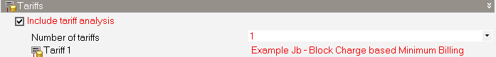
2. The Tariff tab should be the same as for the previous example, J.a. Ratchet Multiplier and Offset
3. On the Charge tab:
Set the Number of charges to 1
Under the Charge 1 settings header:
Set Simple or Block? to 2-Block
Set Charge variable name to DemandCost
Set Source variable to BillingDemand
Set Season to 1-Annual
Set Category variable name to 2-DemandCharges
Leave Remaining into variable blank
Under the Block size multiplier or variable name header, set Use value or variable name? to 1-Value and the Input multiplier value to 1
Set Number of blocks to 3
Set Block size 1 value to 1
Set Block 1 cost per unit value to 25
Set Block size 2 value to 499
Set Block 2 cost per unit value to 0
Set Block size 3 variable name to remaining
Set Block 3 cost per unit value to 0.05
The screenshot below shows how the charge tab should look when you have finished.
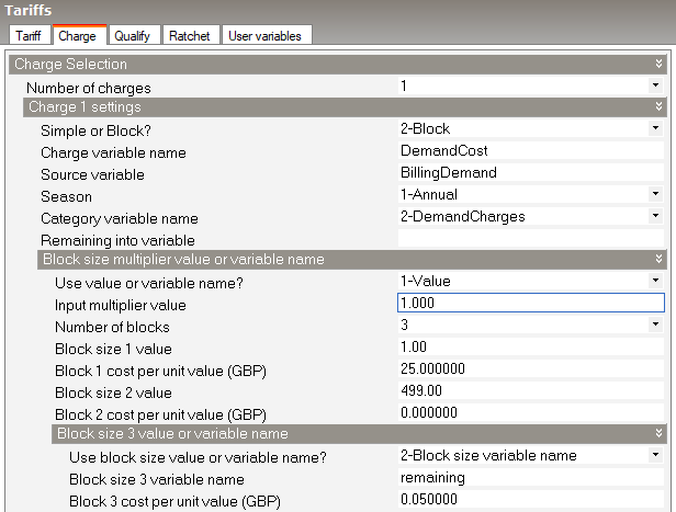
4. On the Ratchet tab:
Set the Number of ratchets to 1.
Under the Ratchet 1 settings header:
Set Ratchet variable name to BillingDemandA
Set Baseline source variable to TotalDemand
Set Adjustment source variable to TotalDemand
Set Season from to 1-Annual
Set Season to to 1-Annual
Under the Multiplier value or variable name header, set Use value or variable name? to 1-Value
Under the Multiplier value or variable name header, set Input multiplier value to 1
Under the Offset value or variable name header, set Use value or variable name? to 1-Value
Under the Offset value or variable name header, set Input offset value to 0
The Ratchet tab should now look similar to the screenshot below.

Report: Economics Results Summary Report
For: Entire Facility
Timestamp: 2025-10-17 13:35:53
Annual Cost
| Electricity | Natural Gas | Other | Total | |
| Cost [£] | 300.00 | 0.00 | 0.00 | 300.00 |
| Cost per Total Building Area [£/m2] | 1.64 | 0.00 | 0.00 | 1.64 |
| Cost per Net Conditioned Building Area [£/m2] | 1.64 | 0.00 | 0.00 | 1.64 |
Tariff Summary
| Selected | Qualified | Meter | Buy or Sell | Group | Annual Cost (£) | |
| EXAMPLE JB - BLOCK CHARGE BASED MINIMUM BILLING | Yes | Yes | ELECTRICITY:FACILITY | Buy | (none) | 300.00 |
Report: Tariff Report
For: EXAMPLE JB - BLOCK CHARGE BASED MINIMUM BILLING
Timestamp: 2025-10-17 13:35:53
General
| Parameter | |
| Meter | ELECTRICITY:FACILITY |
| Selected | Yes |
| Group | (none) |
| Qualified | Yes |
| Disqualifier | n/a |
| Computation | automatic |
| Units | kWh |
Categories
| Jan | Feb | Mar | Apr | May | Jun | Jul | Aug | Sep | Oct | Nov | Dec | Sum | Max | |
| EnergyCharges (£) | 0.00 | 0.00 | 0.00 | 0.00 | 0.00 | 0.00 | 0.00 | 0.00 | 0.00 | 0.00 | 0.00 | 0.00 | 0.00 | 0.00 |
| DemandCharges (£) | 25.00 | 25.00 | 25.00 | 25.00 | 25.00 | 25.00 | 25.00 | 25.00 | 25.00 | 25.00 | 25.00 | 25.00 | 300.00 | 25.00 |
| ServiceCharges (£) | 0.00 | 0.00 | 0.00 | 0.00 | 0.00 | 0.00 | 0.00 | 0.00 | 0.00 | 0.00 | 0.00 | 0.00 | 0.00 | 0.00 |
| Basis (£) | 25.00 | 25.00 | 25.00 | 25.00 | 25.00 | 25.00 | 25.00 | 25.00 | 25.00 | 25.00 | 25.00 | 25.00 | 300.00 | 25.00 |
| Adjustment (£) | 0.00 | 0.00 | 0.00 | 0.00 | 0.00 | 0.00 | 0.00 | 0.00 | 0.00 | 0.00 | 0.00 | 0.00 | 0.00 | 0.00 |
| Surcharge (£) | 0.00 | 0.00 | 0.00 | 0.00 | 0.00 | 0.00 | 0.00 | 0.00 | 0.00 | 0.00 | 0.00 | 0.00 | 0.00 | 0.00 |
| Subtotal (£) | 25.00 | 25.00 | 25.00 | 25.00 | 25.00 | 25.00 | 25.00 | 25.00 | 25.00 | 25.00 | 25.00 | 25.00 | 300.00 | 25.00 |
| Taxes (£) | 0.00 | 0.00 | 0.00 | 0.00 | 0.00 | 0.00 | 0.00 | 0.00 | 0.00 | 0.00 | 0.00 | 0.00 | 0.00 | 0.00 |
| Total (£) | 25.00 | 25.00 | 25.00 | 25.00 | 25.00 | 25.00 | 25.00 | 25.00 | 25.00 | 25.00 | 25.00 | 25.00 | 300.00 | 25.00 |
Charges
| Jan | Feb | Mar | Apr | May | Jun | Jul | Aug | Sep | Oct | Nov | Dec | Sum | Max | Category | |
| DEMANDCOST (£) | 25.00 | 25.00 | 25.00 | 25.00 | 25.00 | 25.00 | 25.00 | 25.00 | 25.00 | 25.00 | 25.00 | 25.00 | 300.00 | 25.00 | DemandCharges |
Corresponding Sources for Charges
| Jan | Feb | Mar | Apr | May | Jun | Jul | Aug | Sep | Oct | Nov | Dec | Sum | Max | |
| BILLINGDEMAND | 7.96 | 7.96 | 7.96 | 7.96 | 7.96 | 7.96 | 7.96 | 7.96 | 7.96 | 7.96 | 7.96 | 7.96 | 95.52 | 7.96 |
Ratchets
| Jan | Feb | Mar | Apr | May | Jun | Jul | Aug | Sep | Oct | Nov | Dec | Sum | Max | |
| BILLINGDEMAND | 7.96 | 7.96 | 7.96 | 7.96 | 7.96 | 7.96 | 7.96 | 7.96 | 7.96 | 7.96 | 7.96 | 7.96 | 95.52 | 7.96 |
Qualifies
| Jan | Feb | Mar | Apr | May | Jun | Jul | Aug | Sep | Oct | Nov | Dec | Sum | Max |
Native Variables
| Jan | Feb | Mar | Apr | May | Jun | Jul | Aug | Sep | Oct | Nov | Dec | Sum | Max | |
| TotalEnergy | 1261.35 | 1113.04 | 1213.71 | 1435.50 | 1696.34 | 1524.70 | 1853.15 | 1732.16 | 1511.94 | 1442.50 | 1182.46 | 1215.03 | 17181.89 | 1853.15 |
| TotalDemand | 4.07 | 5.39 | 5.82 | 6.17 | 6.77 | 7.55 | 7.63 | 7.96 | 6.67 | 6.12 | 5.64 | 4.07 | 73.85 | 7.96 |
| PeakEnergy | 1261.35 | 1113.04 | 1213.71 | 1435.50 | 1696.34 | 1524.70 | 1853.15 | 1732.16 | 1511.94 | 1442.50 | 1182.46 | 1215.03 | 17181.89 | 1853.15 |
| PeakDemand | 4.07 | 5.39 | 5.82 | 6.17 | 6.77 | 7.55 | 7.63 | 7.96 | 6.67 | 6.12 | 5.64 | 4.07 | 73.85 | 7.96 |
| ShoulderEnergy | 0.00 | 0.00 | 0.00 | 0.00 | 0.00 | 0.00 | 0.00 | 0.00 | 0.00 | 0.00 | 0.00 | 0.00 | 0.00 | 0.00 |
| ShoulderDemand | 0.00 | 0.00 | 0.00 | 0.00 | 0.00 | 0.00 | 0.00 | 0.00 | 0.00 | 0.00 | 0.00 | 0.00 | 0.00 | 0.00 |
| OffPeakEnergy | 0.00 | 0.00 | 0.00 | 0.00 | 0.00 | 0.00 | 0.00 | 0.00 | 0.00 | 0.00 | 0.00 | 0.00 | 0.00 | 0.00 |
| OffPeakDemand | 0.00 | 0.00 | 0.00 | 0.00 | 0.00 | 0.00 | 0.00 | 0.00 | 0.00 | 0.00 | 0.00 | 0.00 | 0.00 | 0.00 |
| MidPeakEnergy | 0.00 | 0.00 | 0.00 | 0.00 | 0.00 | 0.00 | 0.00 | 0.00 | 0.00 | 0.00 | 0.00 | 0.00 | 0.00 | 0.00 |
| MidPeakDemand | 0.00 | 0.00 | 0.00 | 0.00 | 0.00 | 0.00 | 0.00 | 0.00 | 0.00 | 0.00 | 0.00 | 0.00 | 0.00 | 0.00 |
| PeakExceedsOffPeak | 4.07 | 5.39 | 5.82 | 6.17 | 6.77 | 7.55 | 7.63 | 7.96 | 6.67 | 6.12 | 5.64 | 4.07 | 73.85 | 7.96 |
| OffPeakExceedsPeak | 0.00 | 0.00 | 0.00 | 0.00 | 0.00 | 0.00 | 0.00 | 0.00 | 0.00 | 0.00 | 0.00 | 0.00 | 0.00 | 0.00 |
| PeakExceedsMidPeak | 4.07 | 5.39 | 5.82 | 6.17 | 6.77 | 7.55 | 7.63 | 7.96 | 6.67 | 6.12 | 5.64 | 4.07 | 73.85 | 7.96 |
| MidPeakExceedsPeak | 0.00 | 0.00 | 0.00 | 0.00 | 0.00 | 0.00 | 0.00 | 0.00 | 0.00 | 0.00 | 0.00 | 0.00 | 0.00 | 0.00 |
| PeakExceedsShoulder | 4.07 | 5.39 | 5.82 | 6.17 | 6.77 | 7.55 | 7.63 | 7.96 | 6.67 | 6.12 | 5.64 | 4.07 | 73.85 | 7.96 |
| ShoulderExceedsPeak | 0.00 | 0.00 | 0.00 | 0.00 | 0.00 | 0.00 | 0.00 | 0.00 | 0.00 | 0.00 | 0.00 | 0.00 | 0.00 | 0.00 |
| IsWinter | 1.00 | 1.00 | 1.00 | 1.00 | 1.00 | 1.00 | 1.00 | 1.00 | 1.00 | 1.00 | 1.00 | 1.00 | 12.00 | 1.00 |
| IsNotWinter | 0.00 | 0.00 | 0.00 | 0.00 | 0.00 | 0.00 | 0.00 | 0.00 | 0.00 | 0.00 | 0.00 | 0.00 | 0.00 | 0.00 |
| IsSpring | 0.00 | 0.00 | 0.00 | 0.00 | 0.00 | 0.00 | 0.00 | 0.00 | 0.00 | 0.00 | 0.00 | 0.00 | 0.00 | 0.00 |
| IsNotSpring | 1.00 | 1.00 | 1.00 | 1.00 | 1.00 | 1.00 | 1.00 | 1.00 | 1.00 | 1.00 | 1.00 | 1.00 | 12.00 | 1.00 |
| IsSummer | 0.00 | 0.00 | 0.00 | 0.00 | 0.00 | 0.00 | 0.00 | 0.00 | 0.00 | 0.00 | 0.00 | 0.00 | 0.00 | 0.00 |
| IsNotSummer | 1.00 | 1.00 | 1.00 | 1.00 | 1.00 | 1.00 | 1.00 | 1.00 | 1.00 | 1.00 | 1.00 | 1.00 | 12.00 | 1.00 |
| IsAutumn | 0.00 | 0.00 | 0.00 | 0.00 | 0.00 | 0.00 | 0.00 | 0.00 | 0.00 | 0.00 | 0.00 | 0.00 | 0.00 | 0.00 |
| IsNotAutumn | 1.00 | 1.00 | 1.00 | 1.00 | 1.00 | 1.00 | 1.00 | 1.00 | 1.00 | 1.00 | 1.00 | 1.00 | 12.00 | 1.00 |
| PeakAndShoulderEnergy | 1261.35 | 1113.04 | 1213.71 | 1435.50 | 1696.34 | 1524.70 | 1853.15 | 1732.16 | 1511.94 | 1442.50 | 1182.46 | 1215.03 | 17181.89 | 1853.15 |
| PeakAndShoulderDemand | 4.07 | 5.39 | 5.82 | 6.17 | 6.77 | 7.55 | 7.63 | 7.96 | 6.67 | 6.12 | 5.64 | 4.07 | 73.85 | 7.96 |
| PeakAndMidPeakEnergy | 1261.35 | 1113.04 | 1213.71 | 1435.50 | 1696.34 | 1524.70 | 1853.15 | 1732.16 | 1511.94 | 1442.50 | 1182.46 | 1215.03 | 17181.89 | 1853.15 |
| PeakAndMidPeakDemand | 4.07 | 5.39 | 5.82 | 6.17 | 6.77 | 7.55 | 7.63 | 7.96 | 6.67 | 6.12 | 5.64 | 4.07 | 73.85 | 7.96 |
| ShoulderAndOffPeakEnergy | 0.00 | 0.00 | 0.00 | 0.00 | 0.00 | 0.00 | 0.00 | 0.00 | 0.00 | 0.00 | 0.00 | 0.00 | 0.00 | 0.00 |
| ShoulderAndOffPeakDemand | 0.00 | 0.00 | 0.00 | 0.00 | 0.00 | 0.00 | 0.00 | 0.00 | 0.00 | 0.00 | 0.00 | 0.00 | 0.00 | 0.00 |
| PeakAndOffPeakEnergy | 1261.35 | 1113.04 | 1213.71 | 1435.50 | 1696.34 | 1524.70 | 1853.15 | 1732.16 | 1511.94 | 1442.50 | 1182.46 | 1215.03 | 17181.89 | 1853.15 |
| PeakAndOffPeakDemand | 4.07 | 5.39 | 5.82 | 6.17 | 6.77 | 7.55 | 7.63 | 7.96 | 6.67 | 6.12 | 5.64 | 4.07 | 73.85 | 7.96 |
| RealTimePriceCosts | 0.00 | 0.00 | 0.00 | 0.00 | 0.00 | 0.00 | 0.00 | 0.00 | 0.00 | 0.00 | 0.00 | 0.00 | 0.00 | 0.00 |
| AboveCustomerBaseCosts | 0.00 | 0.00 | 0.00 | 0.00 | 0.00 | 0.00 | 0.00 | 0.00 | 0.00 | 0.00 | 0.00 | 0.00 | 0.00 | 0.00 |
| BelowCustomerBaseCosts | 0.00 | 0.00 | 0.00 | 0.00 | 0.00 | 0.00 | 0.00 | 0.00 | 0.00 | 0.00 | 0.00 | 0.00 | 0.00 | 0.00 |
| AboveCustomerBaseEnergy | 0.00 | 0.00 | 0.00 | 0.00 | 0.00 | 0.00 | 0.00 | 0.00 | 0.00 | 0.00 | 0.00 | 0.00 | 0.00 | 0.00 |
| BelowCustomerBaseEnergy | 0.00 | 0.00 | 0.00 | 0.00 | 0.00 | 0.00 | 0.00 | 0.00 | 0.00 | 0.00 | 0.00 | 0.00 | 0.00 | 0.00 |
Another source of examples is the large set of tariff input objects provided with EnergyPlus in the macro data set file called “UtilityTariffObjects.imf” located in the “MacroDataSets” folder where EnergyPlus is installed. This file contains sets of objects in EnergyPlus' IDF file format that define tariffs for commercial customers from a collection of U.S. utility companies in August 2005.